The chi-square goodness-of-fit test

When to use this test:

The \(\chi^2\) goodness-of-fit test (Chi-square goodness-of-fit test), also called the one-sample \(\chi^2\) test, is designed to test the agreement of the values observed for \(r\) (\(r\geq2\)) categories \(X_1, X_2,..., X_r\) of a single feature \(X\) with hypothetical expected values for that feature. The values of all \(n\) measurements should be gathered into a table consisting of \(r\) rows (categories: \(X_1, X_2, ..., X_r\)). For each category \(X_i\), we record the frequency of its occurrence \(O_i\), and either the frequency expected for it \(E_i\), or the probability of its occurrence \(p_i\). The expected frequency is calculated as the product \(E_i=np_i\). The resulting table can take one of the forms below.

Assumptions

measurement on a nominal scale – any ordering of the categories is not taken into account,
large expected frequencies, according to the Cochran interpretation (1952)[41],
the sum of the observed frequencies should equal the sum of the expected frequencies, and the sum of all probabilities \(p_i\) should equal 1.

Note!

The table of data can take one of the following forms:

Category \(X_i\)	\(O_i\)	\(E_i\)
\(X_1\)	\(O_1\)	\(E_i\)
\(X_2\)	\(O_2\)	\(E_2\)
...	...	...
\(X_r\)	\(O_r\)	\(E_r\)

Category \(X_i\)	\(O_i\)	\(p_i\)
\(X_1\)	\(O_1\)	\(p_1\)
\(X_2\)	\(O_2\)	\(p_2\)
...	...	...
\(X_r\)	\(O_r\)	\(p_r\)

How to set up the analysis

Statistics \(\to\) Nonparametric tests \(\to\) Chi-square (or via the Wizard).

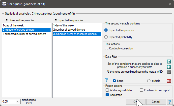
Performing and interpreting the analysis

Example 1. (dinners.pqs file)
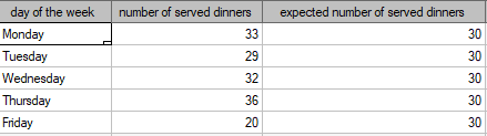
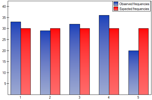
We would like to find out whether the number of dinners served on successive days of the week (Monday to Friday) in a certain school canteen is statistically the same. To do this, a one-week sample was taken, and the number of dinners served was recorded for each day: Monday – 33, Tuesday – 29, Wednesday – 32, Thursday – 36, Friday – 20.

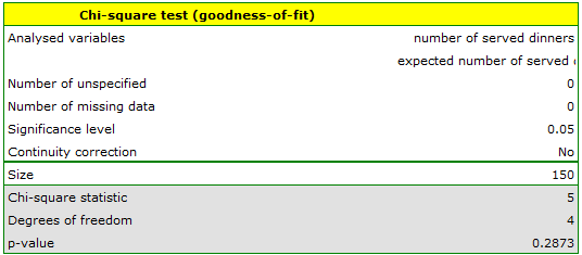
In total, 150 dinners were served over the whole week (5 days). We assume that the probability of a dinner being served is the same on each day, i.e. it equals \(\frac{1}{5}\). The expected number of dinners served for each of the five days of the week is therefore \(E_i=150\cdot\frac{1}{5}=30\).

\(p=0.287297\) for \(df=4\) (not statistically significant, \(\alpha=0.05\))

There is no reason to reject the null hypothesis that the number of dinners served agrees with the expected number of dinners served on each day.

Note! If we wanted to make a larger number of comparisons within a single study, we could apply the Bonferroni correction[2] or another of the corrections described in the Multiple comparisons section. This correction is used to limit the size of the Type I error committed when we compare the observed and expected values between selected days, e.g.: Fri \(\Longleftrightarrow\) Mon, Fri \(\Longleftrightarrow\) Tue, Fri \(\Longleftrightarrow\) Wed, Fri \(\Longleftrightarrow\) Thu – assuming the comparisons are performed independently. The significance level \(\alpha\) for each comparison is determined according to this correction using the formula \(\alpha=\frac{0.05}{r}\), where \(r\) is the number of comparisons performed – for our example, the significance level for a single comparison under the Bonferroni correction is \(\alpha=\frac{0.05}{4}=0.0125\). It should be remembered, however, that by reducing \(\alpha\) for each comparison, we also reduce the power of the test.

FOR THOSE INTERESTED

Hypotheses:

\[ \begin{array}{cl} \mathcal{H}_0: & O_i=E_i \text{ for all categories,}\\ \mathcal{H}_1: & O_i \neq E_i \text{ for at least one category.} \end{array} \]

Formulas:

The test statistic is defined by:

\[ \chi^2=\sum_{i=1}^r\frac{(O_i-E_i)^2}{E_i}. \]

This statistic asymptotically (for large expected frequencies) has the \(\chi^2\) distribution with the number of degrees of freedom calculated using the formula \(df=(r-1)\).

The \(p\) value, determined on the basis of the test statistic and the \(\chi^2\) distribution, is compared with the significance level \(\alpha\): if \(p \le \alpha\), we reject \(\mathcal{H}_0\) in favor of \(\mathcal{H}_1\); if \(p > \alpha\), there is no reason to reject \(\mathcal{H}_0\).