 PQStat
The ANOVA for dependent groups
When to use this test:
The single-factor repeated-measures analysis of variance, i.e. the ANOVA for dependent groups, lets you check whether the mean value of an analysed feature is the same across at least three measurements taken on the same objects under different conditions (e.g. before treatment, during treatment, and after treatment). The test only indicates whether such differences exist at all – it does not say between which measurements they occur; that is the role of the POST-HOC tests, described below.
Assumptions
- measurement on an interval scale,
- the normal distribution for all variables that are the differences of measurement pairs (or normality of the analysed variable for each measurement),
- a dependent model,
- sphericity: the variances of the differences between all pairs of measurements should be close to each other.
The sphericity assumption is checked using Mauchly's test. When it is not met, use the ANOVA for dependent groups with Epsilon correction and MANOVA.
How to set up the analysis
Statistics \(\to\) Parametric tests \(\to\) ANOVA for dependent groups (or via the Wizard).
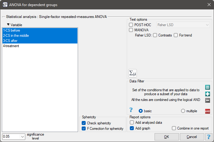
Performing and interpreting the analysis
Since evaluating the result of the ANOVA for dependent groups is inseparable from first checking the sphericity assumption, a full example of performing and interpreting this test – including a situation where the assumption is violated – can be found in the ANOVA for dependent groups with Epsilon correction and MANOVA chapter (see Example 1).
Definitions of measures
Partial \(\eta^2\) – an effect-size measure indicating what proportion of the within-subject variability of the outcomes results from the repeated measurements of the analysed variable, and what proportion remains unexplained. The higher the value, the stronger the association between the measurement and the outcome of the analysed feature.
Hypotheses:
where \(\mu_1\),\(\mu_2\),...,\(\mu_k\) – means of the analysed feature at successive measurements in the population studied.
Formulas: the test statistic is defined by:
where:
\(\displaystyle MS_{BC} = \frac{SS_{BC}}{df_{BC}}\) – mean square between-conditions,
\(\displaystyle MS_{res} = \frac{SS_{res}}{df_{res}}\) – mean square residual,
\(\displaystyle SS_{BC} = \sum_{j=1}^k\left({\frac{\left(\sum_{i=1}^{n}x_{ij}\right)^2}{n}}\right)-\frac{\left(\sum_{j=1}^k{\sum_{i=1}^{n}x_{ij}}\right)^2}{N}\) – between-conditions sum of squares,
\(\displaystyle SS_{res} = SS_{T}-SS_{BS}-SS_{BC}\) – residual sum of squares,
\(\displaystyle SS_{T} = \left(\sum_{j=1}^k{\sum_{i=1}^{n}x_{ij}^2}\right)-\frac{\left(\sum_{j=1}^k{\sum_{i=1}^{n}x_{ij}}\right)^2}{N}\) – total sum of squares,
\(\displaystyle SS_{BS} = \sum_{i=1}^n\left(\frac{\left(\sum_{j=1}^k x_{ij}\right)^2}{k}\right)-\frac{\left(\sum_{j=1}^k{\sum_{i=1}^{n}x_{ij}}\right)^2}{N}\) – between-subjects sum of squares,
\(df_{BC}=k-1\) – degrees of freedom (between-conditions),
\(df_{res}=df_{T}-df_{BC}-df_{BS}\) – degrees of freedom (residual),
\(df_{T}=N-1\) – total degrees of freedom,
\(df_{BS}=n-1\) – degrees of freedom (between-subjects),
\(N=nk\),
\(n\) – sample size,
\(x_{ij}\) – values of the variable for \(i\) subjects \((i=1,2,...n)\) in \(j\) conditions \((j=1,2,...k)\).
The test statistic has the F Snedecor distribution with \(df_{BC}\) and \(df_{res}\) degrees of freedom.
The \(p\) value, determined on the basis of the test statistic, is compared with \(\alpha\): if \(p \le \alpha\), we reject \(\mathcal{H}_0\) in favor of \(\mathcal{H}_1\); if \(p > \alpha\), there is no reason to reject \(\mathcal{H}_0\).
Partial \(\eta^2\)
POST-HOC tests
An introduction to contrasts and POST-HOC tests is provided in section Contrasts and POST-HOC tests, which concerns the one-way analysis of variance for independent groups. The methods below apply analogously to repeated measures (the counts in each measurement are always the same).
The LSD Fisher test
For simple and complex comparisons.
Example – simple comparisons (comparison of 2 selected means):
\(\begin{array}{cc} \mathcal{H}_0: & \mu_j=\mu_{j+1},\\ \mathcal{H}_1: & \mu_j \neq \mu_{j+1}. \end{array}\)
- \(\mathfrak{(i)}\)
The critical difference is calculated using the formula:
\[ CD=\sqrt{F_{\alpha,1,df_{res}}}\cdot \sqrt{\left(\sum_{j=1}^k \frac{c_j^2}{n}\right)MS_{res}}, \]where \(F_{\alpha,1,df_{res}}\) is the critical value (statistic) of the F Snedecor distribution for a given significance level \(\alpha\) and degrees of freedom 1 and \(df_{res}\), respectively.
- \(\mathfrak{(ii)}\)
The test statistic is defined by:
\[ t=\frac{\sum_{j=1}^k c_j\overline{x}_j}{\sqrt{\left(\sum_{j=1}^k \frac{c_j^2}{n}\right)MS_{res}}}. \]The test statistic has the \(t\)-Student distribution with \(df_{res}\) degrees of freedom. For contrasts, \(\sqrt{\left(\sum_{j=1}^k \frac{c_j^2}{n}\right)MS_{res}}\) is replaced by the contrast standard error \(SE_{contrast}\), and the degrees of freedom become \(df_{BS}\).
The Scheffe test
For simple comparisons.
- \(\mathfrak{(i)}\)
The critical difference is calculated using the formula:
\[ CD=\sqrt{F_{\alpha,df_{BC},df_{res}}}\cdot \sqrt{(k-1)\left(\sum_{j=1}^k \frac{c_j^2}{n}\right)MS_{res}}, \]where \(F_{\alpha,df_{BC},df_{res}}\) is the critical value (statistic) of the F Snedecor distribution for a given significance level \(\alpha\) and \(df_{BC}\) and \(df_{res}\) degrees of freedom.
- \(\mathfrak{(ii)}\)
The test statistic is defined by:
\[ F=\frac{\left(\sum_{j=1}^k c_j\overline{x}_j\right)^2}{(k-1)\left(\sum_{j=1}^k \frac{c_j^2}{n}\right)MS_{res}}. \]The test statistic has the F Snedecor distribution with \(df_{BC}\) and \(df_{res}\) degrees of freedom.
The Tukey test
For simple comparisons.
- \(\mathfrak{(i)}\)
The critical difference is calculated using the formula:
\[ CD=\frac{\sqrt{2}\cdot q_{\alpha,df_{res},k} \cdot \sqrt{\left(\sum_{j=1}^k \frac{c_j^2}{n}\right)MS_{res}}}{2}, \]where \(q_{\alpha,df_{res},k}\) is the critical value (statistic) of the studentized range distribution for a given significance level \(\alpha\) and \(df_{res}\) and \(k\) degrees of freedom.
- \(\mathfrak{(ii)}\)
The test statistic is defined by:
\[ q=\sqrt{2}\frac{\sum_{j=1}^k c_j\overline{x}_j}{\sqrt{\left(\sum_{j=1}^k \frac{c_j^2}{n}\right)MS_{res}}}. \]The test statistic has the studentized range distribution with \(df_{res}\) and \(k\) degrees of freedom.
Info. The algorithm for calculating the \(p\) value and the statistic of the studentized range distribution in PQStat is based on Lund's work (1983)[110]. Other applications or web pages may calculate slightly different values than PQStat, since they may be based on less precise or more restrictive algorithms (Copenhaver and Holland (1988), Gleason (1999)).
Test for trend
The test examining the existence of a trend can be calculated in the same situation as the ANOVA for dependent variables, since it is based on the same assumptions, but it captures the alternative hypothesis differently – indicating the existence of a trend in the mean values across successive measurements. The analysis of the trend in the arrangement of means is based on LSD Fisher contrasts. A table of sample contrast values for selected trends can be found in the description of the test for trend for the ANOVA of independent variables.
A linear trend is analyzed based on the linear contrast, assigning appropriate contrast values to the measurements ordered naturally and calculating the LSD Fisher statistic. With the expected direction of the trend known, the alternative hypothesis is one-sided and the one-sided \(p\) value is interpreted; interpreting the two-sided \(p\) value means that the researcher does not know (does not assume) the direction of the possible trend. The determined \(p\) value is compared with \(\alpha\): if \(p \le \alpha\), we reject \(\mathcal{H}_0\) in favor of \(\mathcal{H}_1\); if \(p > \alpha\), there is no reason to reject \(\mathcal{H}_0\).