PROBABILITY DISTRIBUTIONS

What probability distributions are

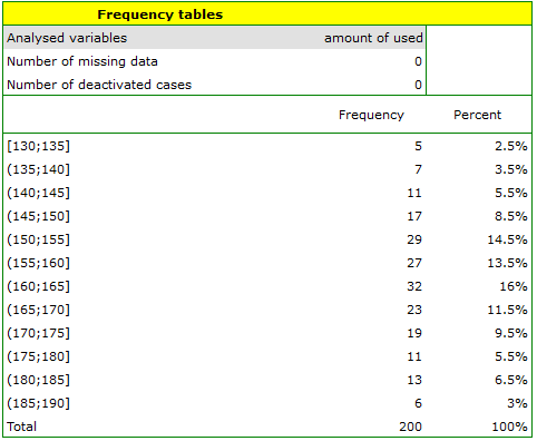
The real distribution of the data from a sample – the empirical data distribution – can be presented by means of Frequency tables (by selecting the Statistics\(\to\)Descriptive analyses\(\to\)Frequency tables menu). For example, the distribution of the number of free minutes used by the subscribers of a certain mobile network operator (example (1), distribution.pqs file) is presented by the following table:

A graphical presentation of the results obtained in the table report is usually made by means of a histogram or a bar chart.

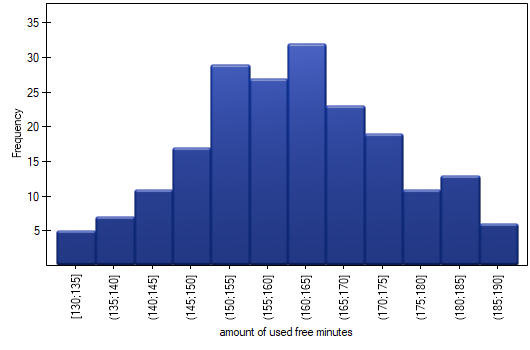
Such a chart can be obtained by ticking the Add chart option in the Frequency tables window.
The theoretical distribution of the data, also called the probability distribution, is usually presented graphically by means of a line chart. Such a line is described by a function (a mathematical model) called the density function of the distribution. The empirical distribution can be replaced by a suitable theoretical distribution – this allows the data to be described by a few parameters instead of listing all the observed values.

Note! To replace an empirical distribution with a theoretical distribution, an intuitive statement of similarity of their shapes is not enough. Specially constructed goodness-of-fit tests are used for this purpose.

The most frequently used probability distribution is the normal distribution (the Gaussian distribution) – and it is exactly such a distribution, with a mean of 161.15 and a standard deviation of 13.03, that is followed by the data on the number of free minutes used (example (1), distribution.pqs file).

CONTINUOUS PROBABILITY DISTRIBUTIONS

Normal distribution (Gaussian distribution)

Also called the bell curve, this is one of the most important distributions in statistics – it has interesting mathematical properties and very often describes phenomena occurring in nature. It is usually denoted by the symbol \(N(\mu,\sigma)\), where \(\mu\) is the expected value (the mean in the population) and \(\sigma\) is the standard deviation – it is exactly these two numbers that fully determine the shape and location of the curve.

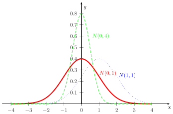
The normal distribution is a distribution symmetrical about a line perpendicular to the x-axis, passing through the point that simultaneously marks the mean, the mode and the median.
The normal distribution with a mean \(\mu=0\) and standard deviation \(\sigma=1\) (\(N(0,1)\)) is the so-called standardised normal distribution.

The t-Student distribution

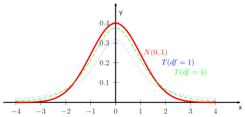
This has a shape similar to the standardised normal distribution, but has longer "tails" – meaning that extreme values occur in it slightly more often. Its shape depends on the number of degrees of freedom \(df\): the more degrees of freedom (i.e. usually the larger the sample), the more the t-Student distribution resembles the normal distribution.

The chi-square distribution (\(\chi^2\))

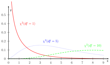
This is a right-skewed distribution (with a longer "tail" on the right side), whose shape depends on the number of degrees of freedom \(df\). As with the t-Student distribution, the shape of the \(\chi^2\) distribution comes to resemble the shape of the normal distribution as the number of degrees of freedom increases.

The Fisher-Snedecor (F) distribution

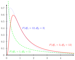
This has a longer right "tail", and its shape depends on two numbers of degrees of freedom: \(df_1\) and \(df_2\). This distribution arises as the ratio of two independent variables with a \(\chi^2\) distribution (each divided by its number of degrees of freedom), and it appears in tests comparing variances or in the analysis of variance (ANOVA).

PROBABILITY DISTRIBUTION CALCULATOR

What it is for

The area under the curve (the density function of the distribution) is the probability \(p\) of occurrence of all possible values of the studied random variable. The whole area under the curve equals \(p=1\). When we want to examine the size of only part of that area, we must give a boundary value called the critical value or the Statistic. For this purpose we use the Probability distribution calculator window. In this window, the value of the area under the curve (\(p\) value) of a given distribution can be calculated on the basis of the Statistic, and likewise the value of the Statistic can be determined on the basis of the \(p\) value.

How to open the calculator

The Probability distribution calculator window is opened by selecting the Statistics\(\to\)Calculators\(\to\)Probability distribution calculator menu.

Example

Example 1. Probability distribution calculator
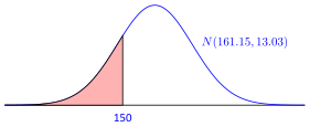
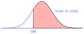
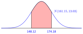
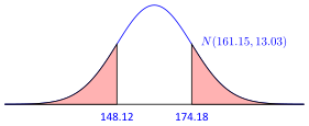
A certain mobile network operator carries out a series of studies on how customers use the number of "free minutes" granted under their subscription. On the basis of a sample of 200 of its customers (in which the distribution of the free minutes used takes the shape of a normal distribution), it determined the mean value \(\overline{x}=161.15\ min.\) and standard deviation \(sd=13.03\ min.\) We want to calculate the probability that a randomly drawn customer used:

150 minutes or less,
more than 150 minutes,
a number of minutes from the interval \([\overline{x}- sd,\overline{x}+ sd] =[148.12\ min.,174.18\ min.]\),
a number of minutes outside the interval \(\overline{x}\pm sd\).

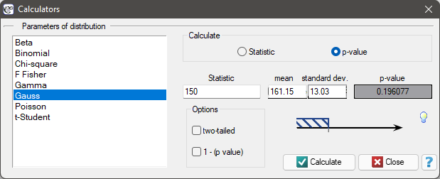
We open the Probability distribution calculator window, select the Gaussian distribution, and enter the mean \(\overline{x}=161.15\ min.\) and standard dev. \(sd=13.03\ min.\), also indicating that we will be calculating the \(p\) value.

To calculate, on the basis of the normal (Gaussian) distribution, the probability that a randomly drawn customer used 150 free minutes or less, we enter the value 150 in the Statistic field. The chosen settings are confirmed with the Calculate button.

The obtained \(p\) value is 0.193961.

Note! Similar calculations can be performed on the basis of the empirical distribution. It is then enough to use the Frequency tables window to determine the percentage of customers using 150 minutes or less (see example (1), distribution.pqs file). In the studied sample of 200 customers, 40 used 150 minutes or less, which is 20% of the sample, so the probability sought is \(P=0.2\).
To calculate, on the basis of the normal (Gaussian) distribution, the probability that a randomly drawn customer used more than 150 free minutes, we enter the value 150 in the Statistic field and tick the 1 - (\(p\) value) option. The chosen settings are confirmed with the Calculate button.

The obtained \(p\) value is 0.806039.
To calculate, on the basis of the normal (Gaussian) distribution, the probability that a randomly drawn customer used a number of minutes from the interval \([\overline{x}- sd,\overline{x}+ sd] =[148.12\ min.,174.18\ min.]\), in the Statistic field we enter one of the interval's end values, and then tick the two-sided option. The chosen settings are confirmed with the Calculate button.

The obtained \(p\) value is 0.682689.
To calculate, on the basis of the normal (Gaussian) distribution, the probability that a randomly drawn customer used a number of minutes outside the interval \([\overline{x}- sd,\overline{x}+ sd] =[148.12\ min.,174.18\ min.]\), in the Statistic field we enter one of the interval's end values, and then tick the options: two-sided and 1 - (\(p\) value). The chosen settings are confirmed with the Calculate button.

The obtained \(p\) value is 0.317311.

FOR THOSE INTERESTED

Normal distribution \(N(\mu,\sigma)\). Formula: the density function is defined as:

\[ f(x,\mu,\sigma)=\frac{1}{\sqrt{2\pi}\sigma}\exp\bigg(-\frac{(x-\mu)^2}{2\sigma^2}\bigg), \]

where:
\(-\infty<x<+\infty\),
\(\mu\) \(-\) the expected value of the population (measured by the mean),
\(\sigma\) \(-\) the standard deviation.

The t-Student distribution. Formula: the density function is defined as:

\[ f(x,df)=\frac{\Gamma(\frac{df+1}{2})}{\Gamma(\frac{df}{2})\sqrt{df\pi}}\left(1+\frac{x^2}{df}\right)^{-\frac{df+1}{2}}, \]

where:
\(-\infty<x<+\infty\),
\(df\) \(-\) degrees of freedom (the sample size decreased by the number of restrictions in the given calculations),
\(\Gamma\) is the Gamma function.

The \(\chi^2\) distribution. Formula: the density function is defined as:

\[ f(x,df)=\frac{1}{2^{\frac{df}{2}}\Gamma{\frac{df}{2}}}x^{\frac{df}{2}-1}e^{-\frac{x}{2}}, \]

where:
\(x>0\),
\(df\) \(-\) degrees of freedom (the sample size decreased by the number of restrictions in the given calculations),
\(\Gamma\) is the Gamma function.

The Fisher-Snedecor (F) distribution. Formula: the density function is defined as:

\[ F(x,df_1,df_2)=\frac{\sqrt{\frac{(df_1x)^{df_1}d_2^{df_2}}{(df_1x+df_2)^{df_1+df_2}}}}{xB\left(\frac{df_1}{2},\frac{df_2}{2}\right)}, \]

where:
\(x>0\),
\(df_1\), \(df_2\) \(-\) degrees of freedom (it is assumed that if \(X\) and \(Y\) are independent with a \(\chi^2\) distribution with, respectively, \(df_1\) and \(df_2\) degrees of freedom, then \(F=\frac{X/df_1}{Y/df_2}\) has the Fisher-Snedecor distribution \(F(df_1,df_2)\)),
\(B\) is the Beta function.