 PQStat
Comparing logistic regression models
When to use:
Because it is possible to analyse many independent variables simultaneously in a single logistic regression model, just as in multiple linear regression, the problem of choosing the optimal model arises. When selecting independent variables, you should keep in mind that the model should contain variables strongly correlated with the dependent variable and weakly correlated with one another.
Comparing logistic regression models lets you answer the question of whether adding (or removing) independent variables significantly changes the quality of the model. If two models do not differ significantly, it is worth choosing the simpler one – the one with fewer variables. In addition, when we are interested in the practical usefulness of a new risk factor, we can compare how much the model's ability to predict the event under study improves once this factor is added.
Assumptions
- the models being compared are built on the same sample (the same observations),
- in the comparison based on the likelihood ratio test, the reduced model is "nested" within the full model, i.e. it is obtained from the full model by removing some of the independent variables,
- in the comparison of predictive value (ROC curves, \(NRI\), \(IDI\)), the predicted probability for both models was determined for the same objects.
Definitions of measures
When comparing models with a different number of independent variables, we pay attention to the model fit and to the information criteria. We decide which model to choose on the basis of the values of \(R_{Pseudo}^2\), \(R^2_{Nagelkerke}\), \(R^2_{Cox-Snell}\) and the result of the likelihood ratio test, which compares successive (neighbouring) models as they are created. For every model the maximum of the likelihood function is calculated, and the likelihood ratio test checks whether the full and reduced models differ significantly in this respect. If the compared models do not differ significantly, we should choose the one with fewer variables – the lack of a difference means that the variables present in the full model but absent from the reduced model do not carry significant information. If, on the other hand, the difference is statistically significant, this means that one of the models (the one with more variables, a larger \(R^2\) and a lower value of the AIC, AICc or BIC information criterion) is significantly better than the other.
Comparing the predictive value of models – the regression models that are built let us predict the probability of the event under study occurring, based on the independent variables analysed. When many factors that increase the risk of the event are already known, an important criterion for a new candidate risk factor is how much it improves prediction performance once it is added to the model. For example, when studying risk factors for coronary heart disease (age, systolic and diastolic blood pressure, obesity, cholesterol, smoking), we can check whether adding a further factor significantly improves the estimation of disease risk. The predictive value of a model follows from the predicted probability determined for every person studied – the closer this value is to 1, the more likely the event is to occur. Based on the predicted probability, we can determine and compare between models the area \(AUC\) under the ROC curve, as well as the \(NRI\) and \(IDI\) coefficients.
- Change in the area under the ROC curve – in logistic regression models the ROC curve is built based on the classification of cases into the group experiencing the event or not, and on the predicted probability of the dependent variable. The larger the area under the curve, the more accurately the probability determined by the model predicts the actual occurrence of the event. By comparing the area under the ROC curve for the full and the reduced model, we therefore check whether adding the factors significantly improved the model's prediction (DeLong's method, described in more detail in the Comparing ROC curves chapter).
Net Reclassification Improvement (\(NRI\)) – a measure based on the reclassification table, describing the upward or downward shift of the predicted probability once a new factor is added to the model. It is determined separately for objects experiencing the event and for those that did not experience it. \(NRI\) can be determined for a given split of the predicted probability into categories (categorical \(NRI\)) or without the need to determine categories (continuous \(NRI\)).
Categorical \(NRI\) requires the split points of the predicted probability to be set arbitrarily (a maximum of 9 points, i.e. a maximum of 10 categories; most often one or two points are used). The values of the categorical \(NRI\) can only be compared with one another when they are based on the same split points. For example, for the split points 0.1 and 0.3: if, in the "old" (smaller) model, a person obtained a probability below 0.1, and in the "new" model – between 0.1 and 0.3, then that person was reclassified upward. If the value from both models falls within the same interval, the person was not reclassified, and if the probability from the "new" model is lower than in the "old" model, we are dealing with a downward reclassification.
regression models reclassification upward no reclassification reclassification downward predicted probability "old" "new" "old" "new" "old" "new" [0.3 to 1] \(\oplus\) [0.1; 0.3) \(\oplus\) \(\oplus\) \(\oplus\) \(\oplus\) [0; 0.1) \(\oplus\) - Continuous \(NRI\) does not require categories to be determined arbitrarily – every change in probability, even the smallest, upward or downward relative to the probability from the "old" model, is treated as a move into the next category.
Note! Using continuous \(NRI\) does not require the arbitrary definition of probability split points, but even small changes in risk (with no counterpart in clinical observation) can influence the value of this coefficient. Categorical \(NRI\), on the other hand, reflects only those changes that the researcher judged to be important when defining the probability split points.The overall \(NRI\) coefficient lies in the range from \(-2\) to \(2\), while the partial coefficients \(NRI_{events}\) and \(NRI_{nonevents}\) lie in the range from \(-1\) to \(1\) (from \(-100\%\) to \(100\%\)). Positive values indicate a favourable reclassification, and negative values – an unfavourable reclassification, as a result of adding the new variable to the model. The statistical significance of the obtained \(NRI\) value is checked with a dedicated Z test.
- Integrated Discrimination Improvement (\(IDI\)) – a coefficient showing the difference between the mean change in predicted probability (between the "old" and "new" model) in the group of objects experiencing the event and the group of objects that did not experience the event. As with \(NRI\), the statistical significance of \(IDI\) is checked with a dedicated Z test.
U-smile – the U-smile method described in the Logistic regression chapter can also be used to compare successive (neighbouring) models: the reference model is the earlier model on the list, and the new model is the next one. The report contains the \(rLR\), \(BA\) or \(RB\) coefficients (to choose from in the AUC-IDI-NRI window) for the four subclasses, the net coefficients for the classes, the overall coefficient, the shares \(I\) and the significance tests; a U-smile plot can be included for each pair. The \(p\) values of the tests assume nested models – for non-nested pairs (the all subsets method) they should be treated as indicative only.
In PQStat, model comparison can be carried out manually or automatically.
Manual model comparison consists of building 2 models:
- the full model – the model with more variables,
- the reduced model – the model with fewer variables; such a model is obtained from the full model by removing the variables that, from the point of view of the phenomenon under study, are superfluous.
The choice of independent variables in the compared models, and then the choice of the better model on the basis of the results of the comparison, is up to the researcher.
Automatic model selection – the program builds successive models itself and indicates the best one according to the chosen criterion.
Model terms. The unit that the automatic methods add to or remove from the model is a term: a single variable, a whole dummy variable (all its 0–1 columns at once) or an interaction. The hierarchy principle applies: an interaction can be in the model only when its main effects are in it, and only the interaction can be removed before them.
The selection criterion is chosen in the analysis window:
- AIC, AICc or BIC – information criteria; the model with the lower value of the criterion is better. A move (adding or removing a term) is accepted only when it lowers the criterion;
- \(p\) of the nested test – the likelihood ratio test comparing the model before and after the change, with a given \(p\) threshold. A term is removed when \(p\) is greater than the threshold, and added when \(p\) is smaller than the threshold. The same \(p\) value is shown in the report as the comparison of neighbouring models;
- validation error – the mean deviance determined on observations that did not take part in fitting the model (described below: Out-of-sample evaluation of models). A move is accepted only when it reduces this error. The criterion requires the Validation option to be switched on – choosing it while validation is off switches cross-validation on.
Selection methods:
- backward elimination – starts from the model with all the variables; in each step the term whose removal lowers the criterion the most is removed; it ends when no removal lowers the criterion any further;
- forward selection – starts from the null model (intercept only); in each step the term that lowers the criterion the most is added; it ends when no addition lowers the criterion any further;
- bidirectional stepwise – starts from the null model; in each step both additions and removals of terms are considered and the best move is chosen; it ends when no move improves the criterion;
- all subsets – all models consistent with the hierarchy principle are fitted (a maximum of 15 terms), and the best model of each size is presented in the report; this method uses the information criteria or the validation error (the \(p\) criterion is not available in it).
All the models are computed on the same set of observations – rows with missing values in any of the candidate variables are discarded once, before the analysis. Thanks to this, the information criteria, the likelihood ratio tests and the comparisons of ROC curves, \(NRI\) and \(IDI\) are comparable between models.
The report contains: the selection method and criterion, the number of terms and of fitted models, the information criteria of the null model, the successive models of the selection path (each with the value of \(-2\ln L\), the AIC, AICc and BIC criteria, the \(R_{Pseudo}^2\), \(R^2_{Nagelkerke}\) and \(R^2_{Cox-Snell}\) coefficients, and the table of coefficients and odds ratios) and the comparison of each neighbouring pair of models with the likelihood ratio test (the \(\chi^2\) statistic, degrees of freedom, \(p\) value). If the evaluation of predictive value was selected in the analysis window, the comparison of ROC curves, \(NRI\) and \(IDI\) are also determined for each neighbouring pair of models – regardless of whether the models are nested. The best model according to the chosen criterion is marked in the report. If no term improves the null model, the report states that the null model is the best. With the all subsets method, neighbouring models may not be nested – in that case the likelihood ratio test is not performed.
Note! The \(p\) values and confidence intervals in an automatically selected model are too optimistic, because the same data set was used both to select the variables and to estimate their effects. Automatic selection should be treated as an aid in searching for a model, and the final choice should be based on subject-matter knowledge. The selected model should be built again in the Logistic regression window and its quality assessed.
Out-of-sample evaluation of models
The fit measures, the information criteria and the tests, as well as the ROC curves, \(NRI\) and \(IDI\), are determined on the same observations on which the coefficients of the models were estimated. Such an assessment is too optimistic – a model usually predicts new cases worse than its fit would suggest, and the difference grows with the number of variables. For this reason, as in comparing multiple regression models, the analysis window makes it possible to evaluate the models on observations that did not take part in fitting them (the Validation option): \(k\)-fold cross-validation (each model is additionally fitted \(k\) times, each time without one of the \(k\) parts of the data, and evaluated on the part left out) or a random test set (the models are fitted on the training part and evaluated on the test part set aside). The split is random, determined by the Seed, and stratified by the dependent variable: the observations with and without the event are split separately, so that the percentage of events is similar in every part.
For each model the report then gives three additional measures:
- mean deviance (\(-2\ln L/n\)) – the value of \(-2\ln L\) determined from the probabilities predicted out of sample, divided by the number of evaluated observations. The lower it is, the better the model; the measure strongly „penalises” predictions that are confident but wrong. This is the validation error – the best model by validation is indicated according to it, and the validation error selection criterion is based on it;
- AUC – the area under the ROC curve built from the probabilities predicted out of sample; it describes the ability of the model to distinguish new objects with the event from objects without the event (0.5 – a useless model, 1 – perfect discrimination);
- Brier score – the mean squared difference between the predicted probability and the actual outcome (1 – event, 0 – no event)[29]; the lower it is, the better the predictions.
The point of reference is the null model, which assigns to every observation the frequency of the event from the training part – its mean deviance and Brier score are given in the model selection block of the report (the \(AUC\) of such a model is 0.5). The same block indicates the best model by validation – regardless of the selection criterion chosen. Out-of-sample evaluation also works in the manual comparison of models.
When validation is switched on, the comparison of the predictive value of the models (ROC curves, \(NRI\), \(IDI\), U-smile) is also determined from the probabilities predicted out of sample: in cross-validation for all the observations, and with a test set – for the observations of the test set. The report marks this with the row ROC, IDI, NRI, U-smile: validation predictions. These results then show whether the additional variables improve the prediction of new cases, and not only the fit to the data on which the model was built.
How to set up the analysis
Statistics \(\to\) Multivariate models \(\to\) Logistic regression – comparing models.
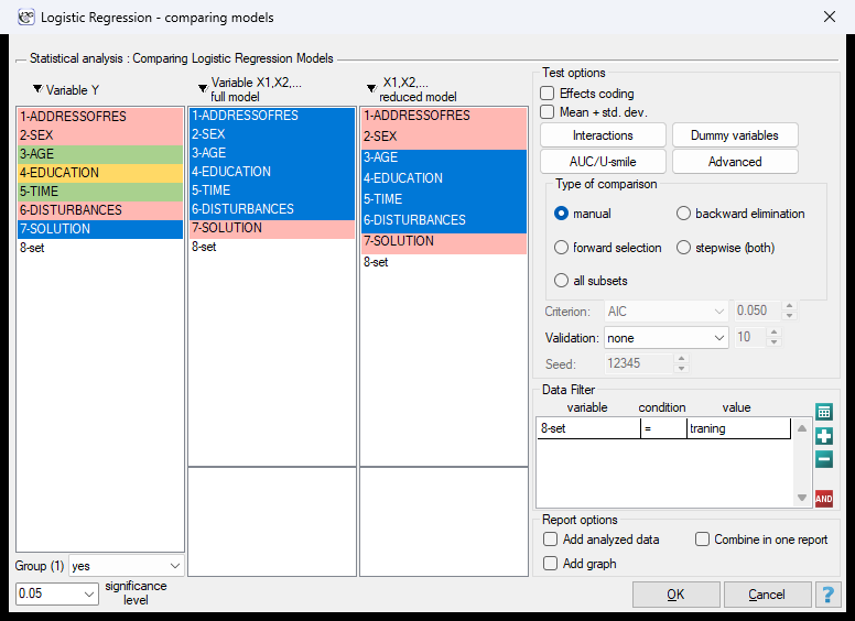
In the window we indicate the dependent variable \(Y\) with the value denoting the event, and the independent variables of the full and the reduced model (in automatic selection – the candidate variables). Model selection options:
- Type of comparison – manual or one of the automatic selection methods,
- Criterion – AIC, AICc, BIC, p (LR / F test) with the threshold given in the adjacent field, or validation error; in the manual mode the criterion is not used,
- Validation – none (evaluation on the training set only), k-fold CV, k = with the number of folds in the adjacent field (from 2 to 100, 10 by default) or test set, % = with the share of the test set as a percentage of the observations (from 5 to 90, 30 by default),
- Seed – the seed of the random split of the data (12345 by default); the same seed means the same split,
- AUC/U-smile – the choice of the comparisons of predictive value (ROC curves, \(NRI\), \(IDI\), U-smile) and of the related plots.
Performing and interpreting the analysis
Continuing example 3 (task.pqs file): in an experiment studying concentration ability, a logistic regression model was built for 130 people from the training set, based on the following variables:
dependent variable: SOLUTION (yes/no) – information about whether the task was solved correctly or not;
independent variables:
ADDRESSOFRES (1=city/0=village),
SEX (1=female/0=male),
AGE (in years),
EDUCATION (1=primary, 2=vocational, 3=secondary, 4=tertiary),
TIME needed to solve the task (in minutes),
DISTURBANCES (1=yes/0=no).
We will check whether all the independent variables are needed in the model.
Manual model comparison
Based on the full model built earlier, we can suspect that the variables ADDRESSOFRES and SEX have little influence on the model built (that is, we cannot successfully classify cases on the basis of them). We will check whether, from a statistical point of view, the full model is better than the model with these two variables removed.
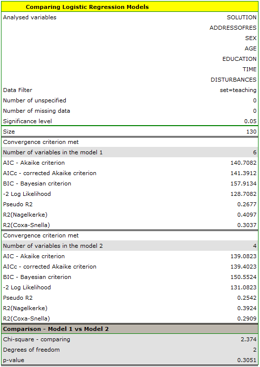
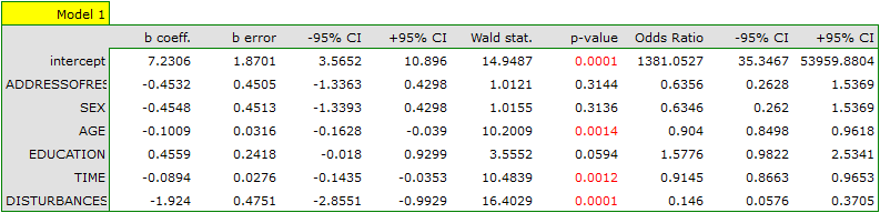

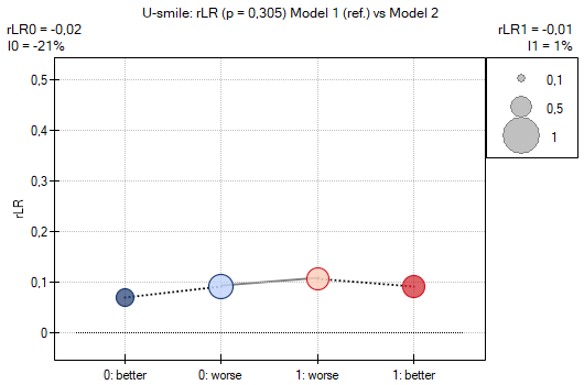
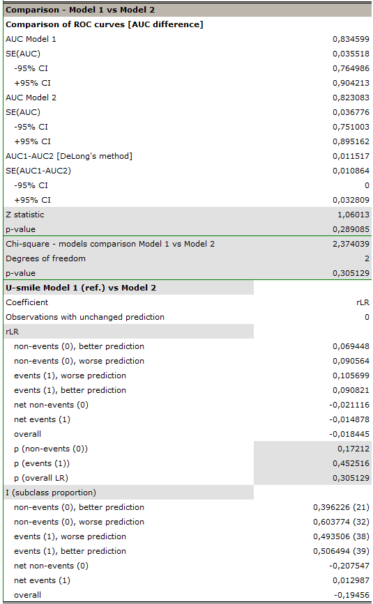
A good illustration of how the likelihood ratio test works is the U-smile plot. We can see that the likelihood of the predictions of the compared models is quite similar – the plot is almost flat (a slightly „sad face”). The smaller model is only non-significantly worse than the larger one – the dashed line in both parts of the plot indicates that the deterioration is statistically non-significant both in the group of people who did not solve the task (the left-hand part of the plot) and in the group of people who solved the task (the right-hand part of the plot).
The two models can also be compared in terms of classification ability by comparing their ROC curves and the \(NRI\) and \(IDI\) values – for this, we select the appropriate option in the analysis window. The resulting report, like the previous one, indicates that the models do not differ in prediction quality, that is, the \(p\) values both for the comparison of ROC curves and for the \(NRI\) and \(IDI\) indices are statistically non-significant. We therefore decide to omit sex and place of residence from the final model.
Out-of-sample evaluation
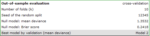
The comparisons above concern the same 130 people on whom both models were fitted. We will check how the models predict the result of people who did not take part in fitting them. In the analysis window we keep the manual comparison of the same two models, and in the Validation field we choose k-fold CV, k = and enter 10 folds (seed 12345).
| training set | cross-validation (\(k=10\)) | |||||
| model | variables | AIC | \(-2\ln L/n\) | mean deviance | AUC | Brier |
| null | 0 | 1.3532 | 0.2418 | |||
| Model 1 (full) | 6 | 140.7082 | 0.9901 | 1.1246 | 0.7856 | 0.1920 |
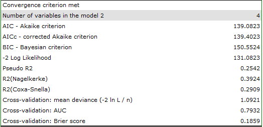
| Model 2 (reduced) | 4 | 139.0823 | 1.0083 | 1.0921 | 0.7932 | 0.1859 |
Both models predict the result much better than the null model (a mean deviance of about 1.1 versus 1.35). At the same time, the values obtained out of sample are clearly worse than the values computed on the training set (for the full model 1.1246 versus \(128.7082/130=0.9901\)) – the assessment on the training data was too optimistic. More importantly, the order of the models is reversed: on the training set the full model is better fitted (like any model with more variables), whereas out of sample the reduced model is better – it has a lower mean deviance (1.0921 versus 1.1246), a larger \(AUC\) (0.7932 versus 0.7856) and a lower Brier score (0.1859 versus 0.1920). Place of residence and sex not only do not significantly improve the fit, but they even slightly worsen the predictions for new people.
Automatic model selection
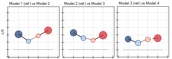
Automatic selection (bidirectional selection, AIC criterion) gives very similar results. The best model is the one built on the independent variables: AGE, EDUCATION, TIME needed to solve the task, DISTURBANCES. The U-smile plots show the individual steps of building the model. In the last step education was added – we can see that it significantly improved only one part of the plot – the one concerning the people who did not solve the task (solid line).
Based on the analyses above, from a statistical point of view, the optimal model is the one containing the 4 most important independent variables: AGE, EDUCATION, TIME needed to solve the task, DISTURBANCES. A detailed analysis of it can be carried out in the Logistic Regression module. However, the final decision as to which model to choose belongs to the researcher.
Example 1. (Heart.pqs file)
Risk factors for a certain heart disease were studied, such as age, BMI, smoking, LDL cholesterol, HDL cholesterol and hypertension. From the researcher's point of view it was of interest to determine how much information about smoking could improve the prediction of the occurrence of the disease under study.
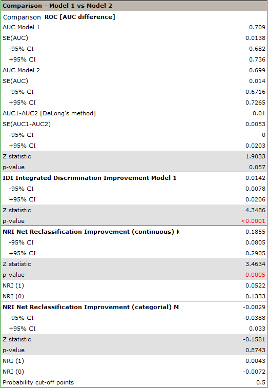
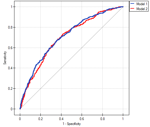
We compare a logistic regression model describing the risk of heart disease based on all the variables studied with a model lacking the smoking information. In the analysis window we select the options related to the evaluation of prediction, that is, the ROC curve and the \(NRI\) coefficients. In addition, we indicate that all the proposed plots should be included in the report.
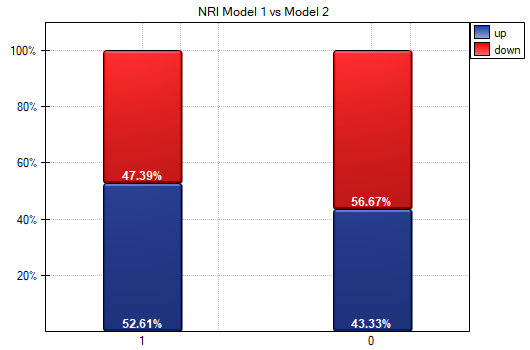
The conclusions drawn from \(NRI\) can also be seen on the plot. An increase in the probability of disease predicted by the model is observed in diseased people (more people were reclassified upward than downward: \(52.61\%\) vs \(47.39\%\)), while a decrease in probability applies to a greater extent to healthy people (more people were reclassified downward than upward: \(56.67\%\) vs \(43.33\%\)).
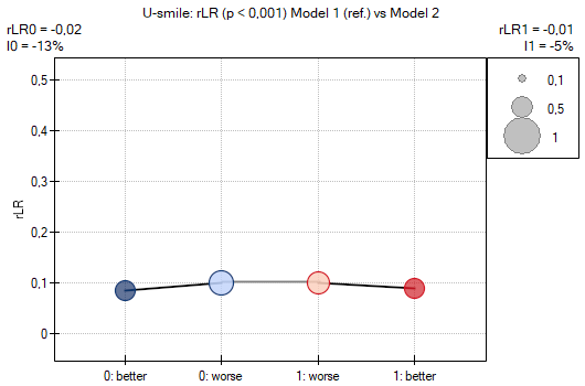
The statistically significant deterioration of the model resulting from removing „smoking” from it is visible in both branches of the U-smile plot and in the fact that all its coefficients are negative.
It is also possible to determine a categorical \(NRI\), but for this we would first need to establish the probability cut-off points, determined by the model, that are accepted in the heart disease literature.
Likelihood ratio test
Hypotheses:
\(\begin{array}{cc} \mathcal{H}_0: & L_{FM}=L_{RM},\\ \mathcal{H}_1: & L_{FM}\ne L_{RM}, \end{array}\)
where \(L_{FM}, L_{RM}\) – the maximum of the likelihood function in the compared models (full and reduced).
Formulas:
The test statistic has the form:
This statistic asymptotically (for large sample sizes) has the \(\chi^2\) distribution with \(df=k_{FM}-k_{RM}\) degrees of freedom, where \(k_{FM}\) and \(k_{RM}\) are the number of estimated parameters in the compared models.
The \(p\) value, determined on the basis of the test statistic, is compared with the significance level \(\alpha\): if \(p \le \alpha\), we reject \(\mathcal{H}_0\) in favor of \(\mathcal{H}_1\); if \(p > \alpha\), there is no reason to reject \(\mathcal{H}_0\).
Out-of-sample evaluation
Let \(\hat{p}_{(-i)}\) denote the probability of the event predicted for observation \(i\) by the model fitted without the part of the data to which observation \(i\) belongs (in cross-validation – without its fold, with a test set – on the training set), and \(y_i\) – the outcome (1 – event, 0 – no event). For the \(n_v\) evaluated observations:
\(AUC\) is the area under the ROC curve determined jointly from all the probabilities \(\hat{p}_{(-i)}\). In the null model \(\hat{p}_{(-i)}\) is the frequency of the event in the corresponding training part. The split is made separately among the observations with and without the event (stratification), as described in the chapter Comparing multiple regression models.
Change in the area under the ROC curve
Hypotheses:
\( \begin{array}{cl} \mathcal{H}_0: & AUC_{FM}=AUC_{RM}, \\ \mathcal{H}_1: & AUC_{FM}\neq AUC_{RM}. \end{array} \)
The method of determining the test statistic, based on DeLong's method, is described in the Comparing ROC curves chapter.
The \(p\) value, determined on the basis of the test statistic, is compared with the significance level \(\alpha\): if \(p \le \alpha\), we reject \(\mathcal{H}_0\) in favor of \(\mathcal{H}_1\); if \(p > \alpha\), there is no reason to reject \(\mathcal{H}_0\).
Net Reclassification Improvement (\(NRI\))
Formulas:
We define:
where:
\(\#events_{up}\) – the number of objects in the group experiencing the event, for whom the predicted probability changed by at least one category upward,
\(\#events_{down}\) – the number of objects in the group experiencing the event, for whom the predicted probability changed by at least one category downward,
\(\#events\) – the number of objects in the group experiencing the event,
\(\#nonevents_{up}\) – the number of objects in the group not experiencing the event, for whom the predicted probability changed by at least one category upward,
\(\#nonevents_{down}\) – the number of objects in the group not experiencing the event, for whom the predicted probability changed by at least one category downward,
\(\#nonevents\) – the number of objects in the group not experiencing the event.
The overall \(NRI\) coefficient and the coefficients expressing the percentage change of classification are determined from the formula:
Interpretation:
The \(NRI_{events}\) coefficient can be interpreted as the net percentage of correctly reclassified people who experienced the event, and \(NRI_{nonevents}\) as the net percentage of correctly reclassified people who did not experience the event. The overall \(NRI\) coefficient is the sum of the \(NRI_{events}\) and \(NRI_{nonevents}\) coefficients, which makes it a coefficient implicitly weighted by the frequency of the event, and it cannot be interpreted as a percentage.
Z test for checking the significance of the \(NRI\) coefficient
Hypotheses:
\( \begin{array}{cl} \mathcal{H}_0: & NRI=0,\\ \mathcal{H}_1: & NRI\neq 0. \end{array} \)
Formulas:
The test statistic has the form:
where:
\( \begin{array}{cl} SE(NRI)= & [\left(\frac{\#events_{up} + \#events_{down}}{\#events^2}-\frac{(\#events_{up} + \#events_{down})^2}{\#events^3}\right)+\\ & +\left(\frac{\#nonevents_{down} + \#nonevents_{up}}{\#nonevents^2}-\frac{(\#nonevents_{down} + \#nonevents_{up})^2}{\#nonevents^3}\right)]^{1/2} \end{array} \)
The \(Z\) statistic asymptotically (for large sample sizes) has the normal distribution.
The \(p\) value, determined on the basis of the test statistic, is compared with the significance level \(\alpha\): if \(p \le \alpha\), we reject \(\mathcal{H}_0\) in favor of \(\mathcal{H}_1\); if \(p > \alpha\), there is no reason to reject \(\mathcal{H}_0\).
Integrated Discrimination Improvement (\(IDI\))
Formulas:
where:
\(\overline{p(diff)}_{events}\) – the mean difference in predicted probability between the regression models ("old" and "new") for the objects that experienced the event,
\(\overline{p(diff)}_{nonevents}\) – the mean difference in predicted probability between the regression models ("old" and "new") for the objects that did not experience the event.
Z test for checking the significance of the \(IDI\) coefficient
Hypotheses:
\( \begin{array}{cl} \mathcal{H}_0: & IDI=0,\\ \mathcal{H}_1: & IDI\neq 0. \end{array} \)
Formulas:
The test statistic has the form:
where:
\(SE(IDI)=\sqrt{\frac{sd(diff)^2_{events}}{\#events}+\frac{sd(diff)^2_{nonevents}}{\#nonevents}}\)
The \(Z\) statistic asymptotically (for large sample sizes) has the normal distribution.
The \(p\) value, determined on the basis of the test statistic, is compared with the significance level \(\alpha\): if \(p \le \alpha\), we reject \(\mathcal{H}_0\) in favor of \(\mathcal{H}_1\); if \(p > \alpha\), there is no reason to reject \(\mathcal{H}_0\).