 PQStat
The ANOVA for independent groups
When to use this test:
The one-way analysis of variance (ANOVA) for independent groups, proposed by Ronald Fisher, lets you check whether the mean value of an analysed feature is the same in at least three independent populations (e.g. groups of patients, product variants, companies). The test only indicates whether such differences exist at all – it does not say between which groups they occur; that is the role of the POST-HOC tests, described in the next section.
Assumptions
- measurement on an interval scale,
- normality of distribution of the analysed variable in each population,
- an independent model,
- equality of variances of the analysed variable across all populations.
When the assumption of equality of variances is not met, use the ANOVA for independent groups with \(F^*\) and \(F''\) corrections.
How to set up the analysis
Statistics \(\to\) Parametric tests \(\to\) ANOVA for independent groups (or via the Wizard).
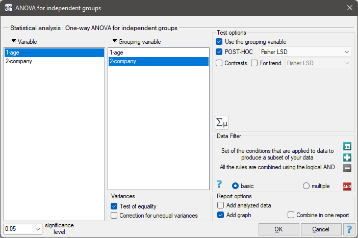
Performing and interpreting the analysis
Example 1. (age ANOVA.pqs file)
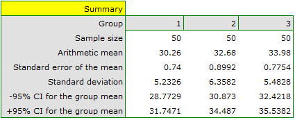
There are 150 people chosen at random from the population of workers of 3 different transport companies. From each company, 50 people are drawn into the sample. Before the experiment begins, we need to check whether the average age of the workers of these companies is similar, since the next stage of the experiment depends on it. The age of each participant is recorded in years.
Age (company 1): 27, 33, 25, 32, 34, 38, 31, 34, 20, 30, 30, 27, 34, 32, 33, 25, 40, 35, 29, 20, 18, 28, 26, 22, 24, 24, 25, 28, 32, 32, 33, 32, 34, 27, 34, 27, 35, 28, 35, 34, 28, 29, 38, 26, 36, 31, 25, 35, 41, 37
Age (company 2): 38, 34, 33, 27, 36, 20, 37, 40, 27, 26, 40, 44, 36, 32, 26, 34, 27, 31, 36, 36, 25, 40, 27, 30, 36, 29, 32, 41, 49, 24, 36, 38, 18, 33, 30, 28, 27, 26, 42, 34, 24, 32, 36, 30, 37, 34, 33, 30, 44, 29
Age (company 3): 34, 36, 31, 37, 45, 39, 36, 34, 39, 27, 35, 33, 36, 28, 38, 25, 29, 26, 45, 28, 27, 32, 33, 30, 39, 40, 36, 33, 28, 32, 36, 39, 32, 39, 37, 35, 44, 34, 21, 42, 40, 32, 30, 23, 32, 34, 27, 39, 37, 35
Before proceeding with the ANOVA analysis, normality of the data distribution was confirmed. The analysis window also tested the assumption of equality of variance, obtaining \(p>0.05\) in both tests.
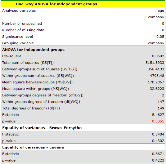
Based on the ANOVA result alone, we do not yet know which companies differ from one another in terms of workers' age – the answer to that question is provided by the POST-HOC analysis, described in the next section.
We can provide a detailed description of the data by selecting Descriptive statistics in the analysis window 
Definitions of measures
Partial \(\eta^2\) – an effect-size measure indicating what proportion of the variability of the analysed feature results from belonging to the compared groups (the factor), and what proportion remains unexplained. The higher the value, the stronger the association between group membership and the outcome of the analysed feature.
Hypotheses:
where \(\mu_1\),\(\mu_2\),...,\(\mu_k\) – means of the analysed variable in the populations from which the samples were drawn.
Formulas: the test statistic is defined by:
where:
\(\displaystyle MS_{BG} = \frac{SS_{BG}}{df_{BG}}\) – mean square between-groups,
\(\displaystyle MS_{WG} = \frac{SS_{WG}}{df_{WG}}\) – mean square within-groups,
\(\displaystyle SS_{BG} = \sum_{j=1}^k{\frac{\left(\sum_{i=1}^{n_j}x_{ij}\right)^2}{n_j}}-\frac{\left(\sum_{j=1}^k{\sum_{i=1}^{n_j}x_{ij}}\right)^2}{N}\) – between-groups sum of squares,
\(\displaystyle SS_{WG} = SS_{T}-SS_{BG}\) – within-groups sum of squares,
\(\displaystyle SS_{T} = \left(\sum_{j=1}^k{\sum_{i=1}^{n_j}x_{ij}^2}\right)-\frac{\left(\sum_{j=1}^k{\sum_{i=1}^{n_j}x_{ij}}\right)^2}{N}\) – total sum of squares,
\(df_{BG}=k-1\) – degrees of freedom (between-groups),
\(df_{WG}=df_{T}-df_{BG}\) – degrees of freedom (within-groups),
\(df_{T}=N-1\) – total degrees of freedom,
\(N=\sum_{j=1}^k n_j\),
\(n_j\) – sample sizes for \((j=1,2,...k)\),
\(x_{ij}\) – values of the variable in the samples for \((i=1,2,...n_j)\), \((j=1,2,...k)\).
The test statistic has the F Snedecor distribution with \(df_{BG}\) and \(df_{WG}\) degrees of freedom.
The \(p\) value, determined on the basis of the test statistic, is compared with the significance level \(\alpha\): if \(p \le \alpha\), we reject \(\mathcal{H}_0\) in favor of \(\mathcal{H}_1\); if \(p > \alpha\), there is no reason to reject \(\mathcal{H}_0\).
Partial \(\eta^2\)
Contrasts and POST-HOC tests
When to use this test:
The ANOVA result only tells us whether there are statistically significant differences among the populations under study – it does not indicate which groups differ. Multiple comparisons answer that question: contrasts (when comparisons are planned in advance, usually only selected ones, so-called a'priori) or POST-HOC tests (when we look for differences only after the ANOVA has been performed, usually between all possible pairs of groups).
Assumptions
- a previously performed ANOVA for independent groups showed a statistically significant difference,
- the choice of method depends on whether the assumption of equality of variances is met: the LSD Fisher, Scheffe and Tukey tests are used when the variances do not differ significantly.
For groups with significantly different variances, use the methods described in the ANOVA for independent groups with \(F^*\) and \(F''\) corrections chapter.
How to set up the analysis
The POST-HOC tests are set up in the same options window used to run the ANOVA for independent groups.
 button.
Performing and interpreting the analysis
Homogeneous groups
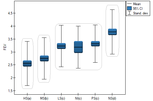
For each post-hoc test, homogeneous groups are constructed. Each homogeneous group represents a set of groups that are not statistically significantly different from each other. For example, suppose we divided subjects into six groups regarding smoking status: Nonsmokers (NS), Passive smokers (PS), Noninhaling smokers (NI), Light smokers (LS), Moderate smokers (MS), Heavy smokers (HS), and we examine their expiratory parameters. In an ANOVA we obtained statistically significant differences in expiratory parameters between the studied groups. To indicate which groups differ significantly and which do not, we perform post-hoc tests. As a result, in addition to the table with the results of each pair of comparisons and the statistical significance expressed as a \(p\) value:
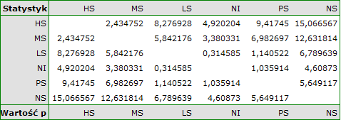
we obtain a division into homogeneous groups:
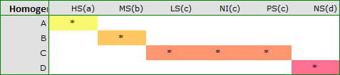
In this case we obtained 4 homogeneous groups, i.e. A, B, C and D, which indicates the possibility of conducting the study based on a smaller division – i.e. instead of the six groups studied originally, further analyses can be conducted based on the four homogeneous groups determined here. The order of the groups was established based on weighted means calculated for each homogeneous group, such that letter A was assigned to the group with the lowest weighted mean, and further letters of the alphabet to groups with progressively higher means.
Continuation of Example 1 (age ANOVA.pqs file): the ANOVA showed a statistically significant difference in the average age of workers of the three transport companies (\(p=0.0051\)). We now check which companies differ from one another in workers' age by performing the Tukey POST-HOC test.
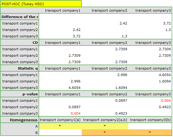
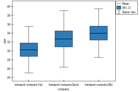
The critical difference (CD) determined for each pair of comparisons is the same (because the group sizes are equal) and equals 2.7309. Comparing the CD value with the value of the mean difference shows that significant differences occur only between the mean age of workers of the first and third transport companies (only for this pair is the CD value smaller than the difference of means). We reach the same conclusion by comparing the \(p\) value of the POST-HOC test with the significance level \(\alpha=0.05\). Workers of the first company are, on average, just over 3 years younger than workers of the third company. Two overlapping homogeneous groups were obtained, which are also marked on the graph.
Test for trend. If, besides the mere existence of differences between groups, we are interested in whether the means change according to a specific, ordered trend (e.g. increase or decrease across successive groups), we can use a variant of the POST-HOC tests based on contrasts – the so-called test for trend. It is run in the same options window as the other POST-HOC tests, by indicating the expected order of the groups. The construction of trend contrasts and the formula for the test statistic are described in the „For those interested” section.
Formulas: the number of all possible simple comparisons is calculated using the formula:
Contrasts
Comparisons within contrasts and POST-HOC tests are written in the form of hypotheses.
The first example – simple comparisons (comparison of 2 selected means):
\(\begin{array}{cc} \mathcal{H}_0: & \mu_1=\mu_2,\\ \mathcal{H}_1: & \mu_1 \neq \mu_2. \end{array}\)
The second example – complex comparisons (comparison of a combination of selected means):
\(\begin{array}{cc} \mathcal{H}_0: & \mu_1=\frac{\mu_2+\mu_3}{2},\\[0.1cm] \mathcal{H}_1: & \mu_1\neq\frac{\mu_2+\mu_3}{2}. \end{array}\)
To define the selected hypotheses, a contrast value \(c_j\), \((j=1,2,...k)\) must be assigned to each mean. The \(c_j\) values are chosen so that the sums for the compared sides are opposite numbers, and their value for means not taking part in the comparison equals 0.
- The first example: \(c_1=1\), \(c_2=-1\), \(c_3=0, ...c_k=0\).
- The second example: \(c_1=2\), \(c_2=-1\), \(c_3=-1\), \(c_4=0\),..., \(c_k=0\).
We can choose the correct hypothesis by:
- \(\mathfrak{(i)}\) Comparing the difference between the selected means with the critical difference (CD) determined by the appropriate POST-HOC test: if the difference of means \(\ge CD\), we reject \(\mathcal{H}_0\) in favor of \(\mathcal{H}_1\); if the difference of means \(< CD\), there is no reason to reject \(\mathcal{H}_0\).
- \(\mathfrak{(ii)}\) Comparing the \(p\) value, determined on the basis of the test statistic of the appropriate POST-HOC test, with \(\alpha\): if \(p \le \alpha\), we reject \(\mathcal{H}_0\) in favor of \(\mathcal{H}_1\); if \(p > \alpha\), there is no reason to reject \(\mathcal{H}_0\).
The LSD Fisher test
For simple and complex comparisons, equal-size groups as well as unequal-size groups, when the variances do not differ significantly.
- \(\mathfrak{(i)}\)
The critical difference is calculated using the formula:
\[ CD=\sqrt{F_{\alpha,1,df_{WG}}}\cdot \sqrt{\left(\sum_{j=1}^k \frac{c_j^2}{n_j}\right)MS_{WG}}, \]where \(F_{\alpha,1,df_{WG}}\) is the critical value (statistic) of the F Snedecor distribution for a given significance level \(\alpha\) and degrees of freedom 1 and \(df_{WG}\), respectively.
- \(\mathfrak{(ii)}\)
The test statistic is defined by:
\[ t=\frac{\sum_{j=1}^k c_j\overline{x}_j}{\sqrt{\left(\sum_{j=1}^k \frac{c_j^2}{n_j}\right)MS_{WG}}}. \]The test statistic has the \(t\)-Student distribution with \(df_{WG}\) degrees of freedom.
The Scheffe test
For simple comparisons, equal-size groups as well as unequal-size groups, when the variances do not differ significantly.
- \(\mathfrak{(i)}\)
The critical difference is calculated using the formula:
\[ CD=\sqrt{F_{\alpha,df_{BG},df_{WG}}}\cdot \sqrt{(k-1)\left(\sum_{j=1}^k \frac{c_j^2}{n_j}\right)MS_{WG}}, \]where \(F_{\alpha,df_{BG},df_{WG}}\) is the critical value (statistic) of the F Snedecor distribution for a given significance level \(\alpha\) and \(df_{BG}\) and \(df_{WG}\) degrees of freedom.
- \(\mathfrak{(ii)}\)
The test statistic is defined by:
\[ F=\frac{\left(\sum_{j=1}^k c_j\overline{x}_j\right)^2}{(k-1)\left(\sum_{j=1}^k \frac{c_j^2}{n_j}\right)MS_{WG}}. \]The test statistic has the F Snedecor distribution with \(df_{BG}\) and \(df_{WG}\) degrees of freedom.
The Tukey test
For simple comparisons, equal-size groups as well as unequal-size groups, when the variances do not differ significantly.
- \(\mathfrak{(i)}\)
The critical difference is calculated using the formula:
\[ CD=\frac{\sqrt{2}\cdot q_{\alpha,df_{WG},k} \cdot \sqrt{\left(\sum_{j=1}^k \frac{c_j^2}{n_j}\right)MS_{WG}}}{2}, \]where \(q_{\alpha,df_{WG},k}\) is the critical value (statistic) of the studentized range distribution for a given significance level \(\alpha\) and \(df_{WG}\) and \(k\) degrees of freedom.
- \(\mathfrak{(ii)}\)
The test statistic is defined by:
\[ q=\sqrt{2}\frac{\sum_{j=1}^k c_j\overline{x}_j}{\sqrt{\left(\sum_{j=1}^k \frac{c_j^2}{n_j}\right)MS_{WG}}}. \]The test statistic has the studentized range distribution with \(df_{WG}\) and \(k\) degrees of freedom.
Info. The algorithm for calculating the \(p\) value and the statistic of the studentized range distribution in PQStat is based on Lund's work (1983)[110]. Other applications or web pages may calculate slightly different values than PQStat, since they may be based on less precise or more restrictive algorithms (Copenhaver and Holland (1988), Gleason (1999)).
Test for trend
The test examining the existence of a trend can be calculated in the same situation as the ANOVA for independent variables, since it is based on the same assumptions, but it captures the alternative hypothesis differently – indicating the existence of a trend in the mean values across successive populations. The analysis of the trend in the arrangement of means is based on LSD Fisher contrasts. By building appropriate contrasts, you can study any type of trend, e.g. linear, quadratic, cubic, etc. Below is a table of sample contrast values for selected trends.
| Contrast | |||||||||||
| Number of groups | Trend | \(c_1\) | \(c_2\) | \(c_3\) | \(c_4\) | \(c_5\) | \(c_6\) | \(c_7\) | \(c_8\) | \(c_9\) | \(c_{10}\) |
| 3 | linear | -1 | 0 | 1 | |||||||
| quadratic | 1 | -2 | 1 | ||||||||
| 4 | linear | -3 | -1 | 1 | 3 | ||||||
| quadratic | 1 | -1 | -1 | 1 | |||||||
| cubic | -1 | 3 | -3 | 1 | |||||||
| 5 | linear | -2 | -1 | 0 | 1 | 2 | |||||
| quadratic | 2 | -1 | -2 | -1 | 2 | ||||||
| cubic | -1 | 2 | 0 | -2 | 1 | ||||||
| 6 | linear | -5 | -3 | -1 | 1 | 3 | 5 | ||||
| quadratic | 5 | -1 | -4 | -4 | -1 | 5 | |||||
| cubic | -5 | 7 | 4 | -4 | -7 | 5 | |||||
| 7 | linear | -3 | -2 | -1 | 0 | 1 | 2 | 3 | |||
| quadratic | 5 | 0 | -3 | -4 | -3 | 0 | 5 | ||||
| cubic | -1 | 1 | 1 | 0 | -1 | -1 | 1 | ||||
| 8 | linear | -7 | -5 | -3 | -1 | 1 | 3 | 5 | 7 | ||
| quadratic | 7 | 1 | -3 | -5 | -5 | -3 | 1 | 7 | |||
| cubic | -7 | 5 | 7 | 3 | -3 | -7 | -5 | 7 | |||
| 9 | linear | -4 | -3 | -2 | -1 | 0 | 1 | 2 | 3 | 4 | |
| quadratic | 28 | 7 | -8 | -17 | -20 | -17 | -8 | 7 | 28 | ||
| cubic | -14 | 7 | 13 | 9 | 0 | -9 | -13 | -7 | 14 | ||
| 10 | linear | -9 | -7 | -5 | -3 | -1 | 1 | 3 | 5 | 7 | 9 |
| quadratic | 6 | 2 | -1 | -3 | -4 | -4 | -3 | -1 | 2 | 6 | |
| cubic | -42 | 14 | 35 | 31 | 12 | -12 | -31 | -35 | -14 | 42 | |
Linear trend
A linear trend, like other trends, can be analyzed by entering the appropriate contrast values. However, if the direction of the linear trend is known, simply use the Linear trend option and indicate the expected order of the populations by assigning them consecutive natural numbers. The analysis is performed based on the linear contrast, i.e. the groups indicated according to the natural order are assigned appropriate contrast values, and the LSD Fisher statistic is calculated.
With the expected direction of the trend known, the alternative hypothesis is one-sided and the one-sided \(p\) value is interpreted. Interpreting the two-sided \(p\) value means that the researcher does not know (does not assume) the direction of the possible trend.
The \(p\) value, determined on the basis of the test statistic, is compared with \(\alpha\): if \(p \le \alpha\), we reject \(\mathcal{H}_0\) in favor of \(\mathcal{H}_1\); if \(p > \alpha\), there is no reason to reject \(\mathcal{H}_0\).