 PQStat
The Kruskal-Wallis ANOVA
When to use this test:
The Kruskal-Wallis one-way analysis of variance by ranks[98][99] is the non-parametric equivalent of the ANOVA for independent groups, extending the Mann-Whitney U test to more than two populations. It lets you check whether the distribution of the analysed feature (most often: its median) is the same in at least three independent populations – it is used instead of the ANOVA for independent groups when that test's assumptions are not met.
Assumptions
- measurement on an ordinal scale or an interval scale,
- an independent model.
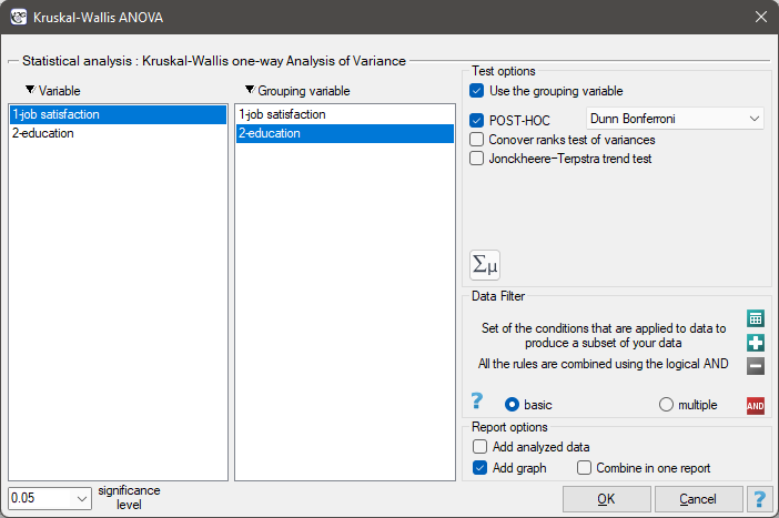
The test assumes that the distributions of the analysed variable in the compared populations have a similar shape – equality of rank variances can be checked with Conover's rank test. If we are interested in a trend in the arrangement of the studied groups, we can additionally perform the Jonckheere-Terpstra test for trend.
How to set up the analysis
Statistics \(\to\) Nonparametric tests \(\to\) Kruskal-Wallis ANOVA (or via the Wizard).
Performing and interpreting the analysis
Example 1. (jobSatisfaction.pqs file)
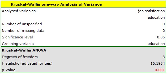
A group of 120 people was surveyed, for whom the job they currently hold is their first job obtained after completing their education. The respondents rated their job satisfaction on a five-point scale, where: 1 – unsatisfying job, 2 – job giving little satisfaction, 3 – job giving an average level of satisfaction, 4 – job giving a fairly high level of satisfaction, 5 – very satisfying job. We will check whether the level of reported job satisfaction differs between education categories.
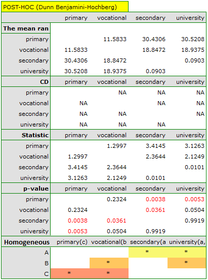
The Dunn POST-HOC analysis with the Bonferroni correction shows that significant differences occur between people with primary and secondary education, and between people with primary and tertiary education. Slightly more differences can be confirmed by choosing the stronger Conover-Iman POST-HOC test.
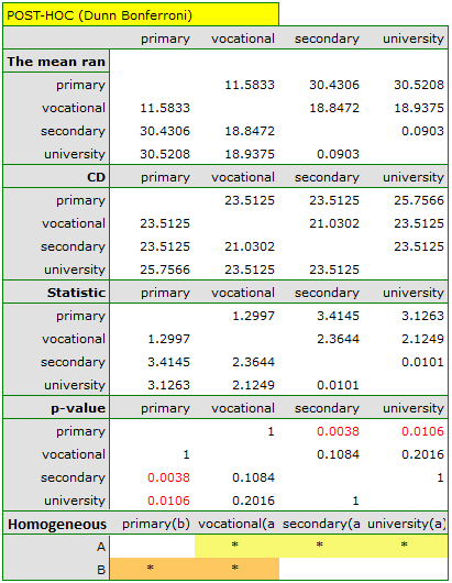
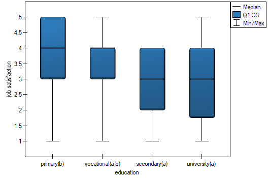
The graph showing medians and quartiles reveals the homogeneous groups determined by the POST-HOC test. For the Dunn result with the Bonferroni correction, two homogeneous groups are visible which are not fully distinct: group (a) – people who rate job satisfaction lower, and group (b) – people who rate it higher. Vocational education belongs to both of these groups, meaning that people with this education rate job satisfaction quite variably.
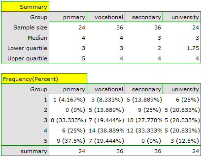
We can provide a detailed description of the data by selecting Descriptive statistics in the analysis window  and choosing to add counts and percentages to the description.
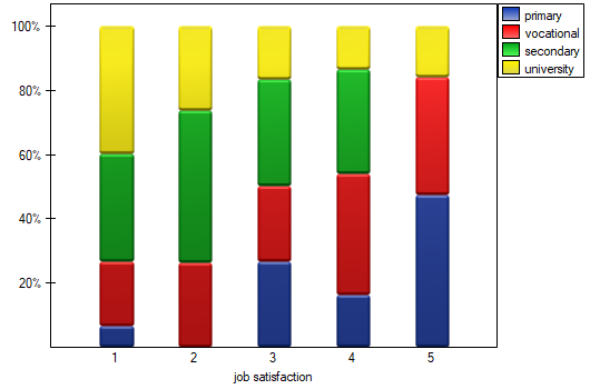
We can also show the distribution of responses in a column chart.
Hypotheses: they relate to the equality of mean ranks for successive populations or are simplified to medians:
where \(\phi_1,\phi_2,...\phi_k\) are the distributions of the analysed variable in the populations from which the samples were drawn.
Formulas: the test statistic is defined by:
where:
\(N=\sum_{j=1}^k n_j\),
\(n_j\) – sample sizes for \((j=1,2,...k)\),
\(R_{ij}\) – ranks assigned to the values of the variable, for \((i=1,2,...n_j)\), \((j=1,2,...k)\),
\(\displaystyle C=1-\frac{\sum(t^3-t)}{N^3-N}\) – correction for ties,
\(t\) – number of cases included in a tie. The correction \(C\) is used when ties occur (otherwise \(C=1\)).
The \(H\) statistic asymptotically (for large sample sizes) has the \(\chi^2\) distribution with \(df=(k-1)\) degrees of freedom.
The \(p\) value, determined on the basis of the test statistic, is compared with \(\alpha\): if \(p \le \alpha\), we reject \(\mathcal{H}_0\) in favor of \(\mathcal{H}_1\); if \(p > \alpha\), there is no reason to reject \(\mathcal{H}_0\).
POST-HOC tests
An introduction to contrasts and POST-HOC tests is provided in section Contrasts and POST-HOC tests, which concerns the one-way analysis of variance.
The Dunn test
For simple comparisons, equal-size groups as well as unequal-size groups (Dunn, 1964[53]). It includes a correction for tied ranks (Zar, 2010[185]) and is corrected for multiple testing – most often with the Bonferroni or Sidak correction (other, newer corrections are described in more detail in the Multiple comparisons section).
- \(\mathfrak{(i)}\)
The critical difference is calculated using the formula:
\[ CD=Z_{\alpha(corrected)}\sqrt{\left(\frac{N(N+1)}{12}-\frac{\sum(t^3-t)}{12(N-1)}\right)\sum_{j=1}^k \frac{c_j^2}{n_j}}, \]where \(t\) is the number of cases included in a tie, and \(Z_{\alpha(corrected)}\) is the critical value (statistic) of the normal distribution for the significance level \(\alpha\) adjusted for the number of possible simple comparisons \(c\) according to the selected correction.
- \(\mathfrak{(ii)}\)
The test statistic is defined by:
\[ Z=\frac{\sum_{j=1}^k c_j\overline{R}_j}{\sqrt{\left(\frac{N(N+1)}{12}-\frac{\sum(t^3-t)}{12(N-1)}\right)\sum_{j=1}^k \frac{c_j^2}{n_j}}}, \]where \(\overline{R}_j\) – mean rank of group \(j\), for \((j=1,2,...k)\). The test statistic asymptotically (for large sample sizes) has the normal distribution, and the \(p\) value is adjusted for the number of possible simple comparisons \(c\) according to the selected correction.
The Conover-Inman test
The non-parametric equivalent of LSD Fisher[48], used for simple comparisons of both equal-size and unequal-size groups.
- \(\mathfrak{(i)}\)
The critical difference is calculated using the formula:
\[ CD=\sqrt{F_{\alpha,1,N-k}}\cdot\sqrt{S^2\frac{N-1-H}{N-k}\sum_{j=1}^k \frac{c_j^2}{n_j}}, \]where \(\displaystyle S^2=\frac{1}{N-1}\left(\sum_{j=1}^k\sum_{i=1}^{n_j}R_{ij}^2-N\frac{(N+1)^2}{4}\right)\), and \(F_{\alpha,1,N-k}\) is the critical value (statistic) of the F Snedecor distribution for a given significance level \(\alpha\) and for degrees of freedom 1 and \(N-k\), respectively.
- \(\mathfrak{(ii)}\)
The test statistic is defined by:
\[ t=\frac{\sum_{j=1}^k c_j\overline{R}_j}{\sqrt{S^2\frac{N-1-H}{N-k}\sum_{j=1}^k \frac{c_j^2}{n_j}}}, \]where \(\overline{R}_j\) – mean rank of group \(j\), for \((j=1,2,...k)\). The test statistic has the \(t\)-Student distribution with \(N-k\) degrees of freedom.