The Conover ranks test of variance

When to use this test:

The Conover squared ranks test lets you check whether the dispersion (variability) of an analysed feature is similar across several populations – similarly to the Fisher-Snedecor test (for two populations) or the Levene and Brown-Forsythe tests (for at least two populations). It is their non-parametric counterpart: it does not assume normality of the data distribution and is based on ranks[48]. It is usually used as a complement to the Kruskal-Wallis ANOVA, since this test examines the variability of the data (distances from the mean) rather than its level.

Assumptions

measurement on an interval scale.

How to set up the analysis

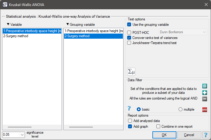
Statistics \(\to\) Nonparametric tests \(\to\) Kruskal-Wallis ANOVA, option Conover ranks test of variance, or Statistics \(\to\) Nonparametric tests \(\to\) Mann-Whitney, option Conover ranks test of variance.

Performing and interpreting the analysis

Example 1. (surgeryMethod.pqs file)
Patients have been prepared for spinal surgery and will be operated on using one of three methods. Each patient has been provisionally assigned to a surgery type. At a later stage we intend to compare patients' condition after surgery, so we want the groups of patients to be comparable – they should be similar, among other things, in terms of the height of the interbody space (WPMT) before surgery. The similarity should concern not only the average values but also the variability of the groups.

The distribution of the data was checked.

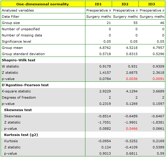
It turns out that for two of the surgery methods, WPMT shows deviations from normality, largely caused by the skewness of the data. We will conduct further comparative analysis using the Kruskal-Wallis test, to check whether the WPMT level differs between the methods, and the Conover test, to indicate whether the spread of WPMT scores is similar for each method.

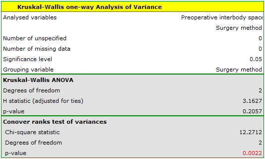
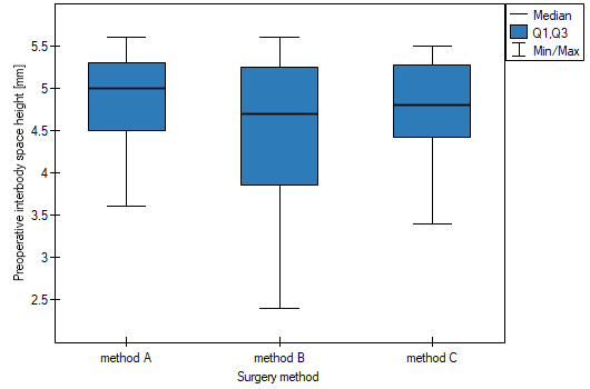
\(p=0.0022\) for the Conover variance test (statistically significant, \(\alpha=0.05\)), \(p=0.2057\) for the Kruskal-Wallis test (not statistically significant)

The WPMT ranges differ significantly between surgery methods, while the WPMT level does not.

We first interpret the result of the Conover variance test, which indicates statistically significant differences in the ranges of the compared groups. The graph suggests that the differences mainly concern group 3. Since differences in WPMT range were detected, the interpretation of the Kruskal-Wallis test result (comparing WPMT levels for these methods) should be cautious, since this test is sensitive to heterogeneity of variance. Although the Kruskal-Wallis test showed no significant differences, it is recommended that patients with low WPMT values (mostly assigned to surgery method B) be distributed more evenly – i.e. that we check whether they could instead be offered surgery method A or C. After reassigning patients, the analysis should be repeated.

FOR THOSE INTERESTED

Hypotheses:

\[\begin{array}{cc} \mathcal{H}_0: & \text{the dispersion of the data in the compared populations is the same, }\\ \mathcal{H}_1: & \text{at least two populations differ in the amount of data dispersion}. \end{array}\]

Formulas: The test statistic is defined by:

\[ \chi^2=\frac{1}{D^2}\left(\sum_{j=1}^k\frac{S_j^2}{n_j}-N\overline{S}^2\right) \]

where:
\(N=n_1+n_2+...+n_k\),
\(n_j\) – size of the individual groups,
\(S_j\) – sum of squared ranks in group \(j\),
\(\overline{S}=\frac{1}{N}\sum_{j=1}^kS_j\) – mean of all squared ranks,
\(D^2=\frac{1}{N-1}\left(\sum_{i=1}^NR_i^4-N\overline{S}^2\right)\),
\(R_i\) – ranks for values representing the distance of the measurement from the mean of a given group.

This statistic has the \(\chi^2\) distribution with \(k-1\) degrees of freedom.

The \(p\) value, determined on the basis of the test statistic, is compared with the significance level \(\alpha\): if \(p \le \alpha\), we reject \(\mathcal{H}_0\) in favor of \(\mathcal{H}_1\); if \(p > \alpha\), there is no reason to reject \(\mathcal{H}_0\).