 PQStat
Hypothesis testing
Generalizing the results obtained for a sample to the whole population essentially falls into 2 parts:
- estimation \(–\) estimating the values of population parameters on the basis of a statistical sample,
- verification of statistical hypotheses \(–\) checking specific assumptions formulated about the parameters of the general population, on the basis of the results obtained from a sample.
Point and interval estimation
In practice, we most often do not know the parameters (characteristics) of the whole population, and have only a sample drawn from that population. Point estimators are characteristics calculated on the basis of a random sample, and their accuracy is described by the standard error. The true value of the population parameter lies in the neighbourhood of the computed point estimator – for example, the population parameter arithmetic mean \(\mu\) lies in the neighbourhood of the sample estimator \(\overline{x}\).
Knowing the theoretical distribution of the estimator, we can, with a predetermined confidence level (\(1-\alpha\)), estimate the value of the population parameter on the basis of the estimator obtained from the random sample. This procedure is called interval estimation, and the interval determined in this way is called the confidence interval; \(\alpha\) itself is called the significance level.
The significance level most commonly used is 0.05, 0.01, or 0.001.
Verification of statistical hypotheses
Verifying statistical hypotheses proceeds in several steps.
Step 1. Formulating the hypotheses. These will be verified using an appropriate statistical test. Every test states a general form of the null hypothesis \(-\) \(\mathcal{H}_0\) (ang. null hypothesis) and the alternative hypothesis \(-\) \(\mathcal{H}_1\) (ang. alternative hypothesis):
\(\begin{array}{cl} \mathcal{H}_0: & \textrm{\textbf{there is no} statistically significant \textbf{difference} between the (means,}\\ &\textrm{medians, proportions, distributions, etc.) of the \textbf{populations}},\\\\ \mathcal{H}_1: & \textrm{\textbf{there is} a statistically significant \textbf{difference} between the means,}\\ &\textrm{medians, proportions, distributions, etc.) of the \textbf{populations}}. \end{array}\)
The researcher must formulate the hypothesis so that it is consistent both with reality and with the requirements of the chosen statistical test, e.g.:
\(\begin{array}{cl} \mathcal{H}_0: & \textrm{the percentage of women and men running a business}\\ &\textrm{in the population studied is the same}. \end{array}\)
If we do not know which percentage (of women or of men) might be higher in the population studied, the alternative hypothesis should be two-sided, i.e. we do not assume the direction of the difference:
\(\begin{array}{cl} \mathcal{H}_1: & \textrm{the percentage of women and men running a business}\\ &\textrm{in the population studied is different}. \end{array}\)
Only in rare cases, when we are certain about the direction of the expected difference, can a one-sided alternative hypothesis be used.
Step 2. Choosing the test and calculating the test statistic. We check which of the hypotheses – \(\mathcal{H}_0\) or \(\mathcal{H}_1\) – is more probable. Depending on the type of study and the nature of the variables, we select an appropriate statistical test.
Note! The choice of statistical test depends above all on the appropriate measurement scale (interval, ordinal, nominal) represented by the data being analysed, as well as on the study's design (dependent or independent model). Measurements of a given feature are called dependent (paired) when they are taken several times for the same objects. When the measurements of a given feature concern objects belonging to different groups, we speak of independent (unpaired) groups. Examples of studies with dependent groups: the body weight of patients before and after a weight-loss therapy, the reaction to a stimulus of the same group of people under two different conditions (e.g. at night and during the day), the assessment of creditworthiness of the same customers carried out by 2 different banks. Examples of studies with independent groups: body weight in a group of healthy patients and a group of ill patients, the effectiveness of fertilization with several different types of fertilizer, the size of GDP in different countries.Note! The graph included in the Wizard window makes it easier to choose the appropriate statistical test.The test statistic of the chosen test, calculated according to its formula, follows a theoretical distribution appropriate to it.
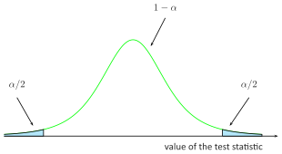
The program calculates the value of the test statistic and the corresponding \(p\) value (i.e. that part of the area under the curve which corresponds to the value of the test statistic). The \(p\) value lets us choose the more probable of the null and alternative hypotheses. In doing so we always assume that the null hypothesis is true, and the data collected are meant to supply sufficient evidence against this hypothesis:
\[ \begin{array}{ccl} \text{ if } p \le \alpha & \Longrightarrow & \text{ we reject } \mathcal{H}_0 \text{ in favor of } \mathcal{H}_1, \\ \text{ if } p > \alpha & \Longrightarrow & \text{ there is no reason to reject } \mathcal{H}_0. \\ \end{array}\]A significance level of \(\alpha=0.05\) is usually adopted, accepting that in 5% of cases we will reject the null hypothesis even though it is true. In special situations a different significance level can be chosen, e.g. 0.01 or 0.001.
- Step 3. Describing the results of the hypothesis verification.
Type I and Type II errors
A statistical test can fail to match reality in two ways:
| reality | |||
| \(\mathcal{H}_0:\) true | \(\mathcal{H}_0:\) false | ||
| test result | \(\mathcal{H}_0:\) true | OK | \(\beta\) |
| \(\mathcal{H}_0:\) false | \(\alpha\) | OK | |
We can make 2 kinds of errors:
- \(\alpha\) = Type I error – the probability of rejecting hypothesis \(\mathcal{H}_0\) when it is true,
- \(\beta\) = Type II error – the probability of accepting hypothesis \(\mathcal{H}_0\) when it is false.
The power of the test is \(1 - \beta\).
The values \(\alpha\) and \(\beta\) are related to each other. Accepted practice is to fix the significance level \(\alpha\) in advance and to minimize \(\beta\) by increasing the sample size.