Multivariate normality tests

When to use:

Many methods of multivariate analysis, including MANOVA, Hotelling's tests, and regression models, are based on the assumption of multivariate normality. If a set of variables is characterised by a multivariate normal distribution, then each variable has a normal distribution. However, when all the individual variables are characterised by a normal distribution, their set need not have a multivariate normal distribution – therefore, testing the univariate normality of each variable may be useful, but cannot be assumed to be sufficient.

Assumptions

measurement on an interval scale for all analysed variables.

Definitions of measures

Different types of statistical analysis that assume normality are sensitive to different degrees to different kinds of departure from this assumption. Tests referring to means in their hypotheses are assumed to be more sensitive to skewness, while tests comparing covariances depend more heavily on kurtosis.

The Mardia test – proposed by Mardia in 1970[118] and modified in 1974[119], this test examines the normality of the distribution by analysing separately the magnitude of multivariate skewness and multivariate kurtosis.

The Jarque-Bera test – Jarque and Bera[90] proposed combining the two Mardia measures (skewness and kurtosis) into a single test.

The Hanusz-Tarasinska test – a similar way of combining skewness and kurtosis information into a single test is provided by the method of Hanusz and Tarasinska (2014)[79].

The Henze-Zirkler test – Henze and Zirkler (1990)[82] proposed a test examining multivariate normality of the distribution, extending the work of Baringhaus and Henze on the empirical characteristic function[56]. In the literature, this test is considered one of the strongest tests dedicated to the multivariate normal distribution (Thode, 2002)[166].

How to set up the analysis

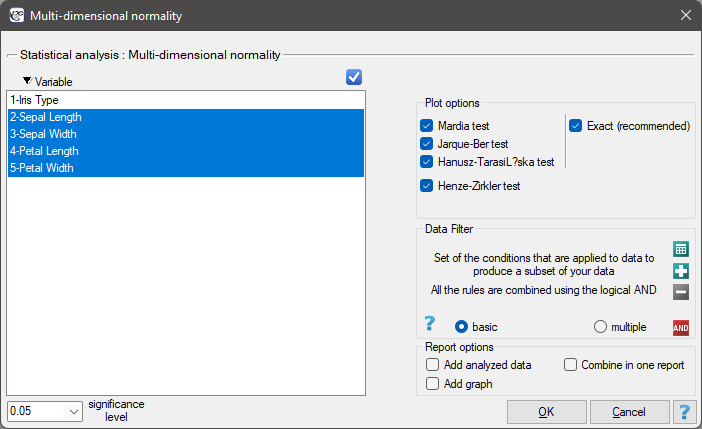
Statistics \(\to\) Normality tests \(\to\) Multi-dimensional normality.

Performing and interpreting the analysis

Example 1. (Iris.pqs file)
We examine the normality of the distribution for the classic data set of R.A. Fisher from 1936[60]. The file is included in the help supplied with the program, and contains measurements of the length and width of the petals and calyx sepals for 3 varieties of iris. The analysis will be performed separately for each variety.

In the analysis window, we select all the tests and the graph, and to repeat the analysis for each iris variety, we set a multiple filter. All the results will be returned to the same worksheet, so we select the Combine into one report option.

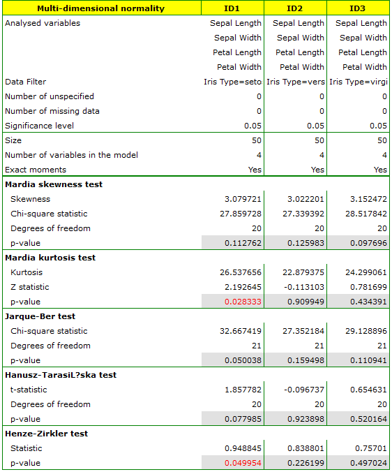
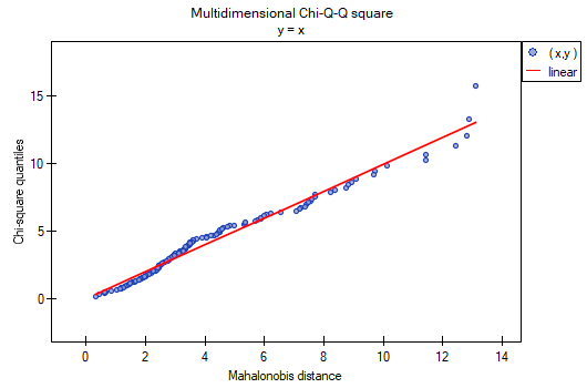
all tests \(p>0.05\) for the versicolor and virginica varieties; borderline results for the setosa variety

The data distribution does not deviate from the multivariate normal distribution for the versicolor and virginica varieties; for the setosa variety, the results are inconclusive.

For the setosa variety, the Mardia kurtosis test and the Henze-Zirkler test indicate deviations from the multivariate normal distribution. We can also observe such deviations on the graph below, where as the Mahalanobis distance increases, the points lie further and further from the straight line.

FOR THOSE INTERESTED

Hypotheses (common to all tests):

\[\begin{array}{cl} \mathcal{H}_0: & \text{the distribution of the data in the population }=\text{ a multivariate normal distribution},\\ \mathcal{H}_1: & \text{the distribution of the data in the population }\neq\text{ a multivariate normal distribution.} \end{array}\]

The Mardia test
Formulas: Mardia defined multivariate skewness and kurtosis as follows:

\[ skew=\frac{1}{n^2}\sum_{i=1}^n\sum_{j=1}^nm_{ij}^3, \quad kurt=\frac{1}{n}\sum_{i=1}^nm_{ii}^2 \]

where:
\(m_{ij}=\left(X_i-\bar{X}\right)^TS^{-1}\left(X_j-\bar{X}\right)\),
\(S=\frac{1}{n}\sum_{j=1}^n\left(X_i-\bar{X}\right)\left(X_i-\bar{X}\right)^T\),
\(\bar{X}\) – the mean, \(S\) – the covariance matrix.
For data coming from a sample rather than a population, the formulas for skewness and kurtosis are multiplied respectively: skewness by \(\left(n/(n-1)\right)^3\), and kurtosis by \(\left(n/(n-1)\right)^2\).

Skewness test: when the sample is drawn from a population with a multivariate normal distribution (null hypothesis), the test statistic is defined by (Mardia, 1970):

\[ \chi^2(M)=\frac{n}{6}skew \]

or, with a correction for exact moments for groups with smaller sample sizes (\(<20\)) (Mardia, 1974):

\[ \chi_c^2(M)=\frac{n}{6}\frac{(n+1)(n+3)(k+1)}{n((n+1)(k+1)-6)}skew \]

This statistic asymptotically (for large sample sizes) has the \(\chi^2\) distribution with \(df=f=\frac{k(k+1)(k+2)}{6}\) degrees of freedom.

Kurtosis test: when the sample is drawn from a population with a multivariate normal distribution (null hypothesis), the test statistic is defined by (Mardia, 1974):

\[ Z(M)=\frac{kurt-k(k+2)}{\sqrt{\frac{8k(k+2)}{n}}} \]

or, with a correction (Mardia, 1974):

\[ Z_c(M)=\frac{(n+1)kurt-k(k+2)(n-1)}{\sqrt{\frac{8k(k+2)(n-3)(n-k-1)(n-k+1)}{(n+3)(n+5)}}} \]

This statistic asymptotically (for large sample sizes) has the normal distribution.

Interpretation: the \(p\) value, determined on the basis of the test statistic, is compared with the significance level \(\alpha\) for both tests (the skewness test and the kurtosis test): if \(p \le \alpha\) for at least one test, we reject \(\mathcal{H}_0\) in favor of \(\mathcal{H}_1\); if \(p > \alpha\) for both tests used, there is no reason to reject \(\mathcal{H}_0\).

The Jarque-Bera test
Formulas: this test is based on the skewness and kurtosis statistics of the Mardia test. The test statistic is defined by:

\[ \chi^2(JB)=\chi^2(M)+(Z(M))^2 \]

or, with a correction (Mardia, 1974):

\[ \chi_c^2(JB)=\chi_c^2(M)+(Z_c(M))^2 \]

This statistic asymptotically (for large sample sizes) has the \(\chi^2\) distribution with \(df=f+1\) degrees of freedom.

The \(p\) value, determined on the basis of the test statistic, is compared with the significance level \(\alpha\): if \(p \le \alpha\), we reject \(\mathcal{H}_0\) in favor of \(\mathcal{H}_1\); if \(p > \alpha\), there is no reason to reject \(\mathcal{H}_0\).

The Hanusz-Tarasinska test
Formulas: this test is based on the skewness and kurtosis statistics of the Mardia test. The test statistic is defined by:

\[ t_c(HT)=\frac{Z_c(M)}{\sqrt{\frac{\chi_c^2(M)}{f}}} \]

The test statistic has the \(t\)-Student distribution with \(df=f\) degrees of freedom.

The Henze-Zirkler test
Formulas: the test statistic is defined by:

\[ Z(HZ)_{\beta}=n\left(4I_E+D_{n,\beta}I_{E^c}\right) \]

where:
\(I_E\) and \(I_{E^c}\) – indicator functions depending on the singularity of the covariance matrix,
\(D_{n,\beta}=\frac{1}{n^2}\sum \exp\left(\frac{-\beta^2||Y_j-Y_k||^2}{2}\right)+(1+2\beta^2)^{-p/2}-2(1+\beta^2)^{-p/2}\sum \exp\left(\frac{-\beta^2||Y_j||^2}{2(1+\beta^2)}\right)\),
\(Y_i=S^{1/2}(X_i-\bar{X})\),
\(\beta*=2^{-1/2}\left(\frac{n(2k+1)}{4}\right)^{1/(k+4)}\) – the optimal value of the parameter \(\beta\).

The statistic \(Z(HZ)_{\beta}\) asymptotically (for large sample sizes) has the normal distribution, based on the mean and variance described by Henze and Zirkler, and is read one-sided.

The one-sided \(p\) value, determined on the basis of the test statistic, is compared with the significance level \(\alpha\): if \(p \le \alpha\), we reject \(\mathcal{H}_0\) in favor of \(\mathcal{H}_1\); if \(p > \alpha\), there is no reason to reject \(\mathcal{H}_0\).