PQStat
DESCRIPTIVE STATISTICS
To conduct Descriptive Statistics on the basis of a Map data we should have at our disposal a point, multipoint, or polygonal file. In the case of an analysis of a polygonal file, calculations are based on centroids of polygons, and in the case of a multipoint file they are based on centers of objects.
Boundaries of an area in which analysed points are enclosed can be defined, depending on a particular need, with the help of: a convex hull, the smallest rectangle, a rectangle from from layer bounding, or the smallest circle. The studied area can also be defined only with the use of the size of its area.
The distance between the points is measured with the Euclidean metric.
The basic statistics made for point analysis:
- \(A\) –the area of a studied region,
- \(n\) –the size of a sample, i.e. the number of points lying within the studied region,
- \(D=\frac{n}{A}\) –density,
descriptive statistics of the distance matrix between points:
- arithmetic mean with confidence interval,
- standard deviation,
- median,
- quartiles,
- minimum and maximum.
The analysis also gives a graph pertaining to a distance matrix and layers which can be drawn on the surface of a map. Layers pertain to centrographic measures: the measure of central tendency and the measure of dispersion:
- The center of point distribution: the mean of coordinates of the \(X\) axis and the \(Y\) axis (\(\overline{x}\), \(\overline{y}\)),
The area of standard deviations, built around the center, defined by:
Circle
The radius of the circle is \(sdd\) –standard distance from the center ( standard distance deviation) expressed with the formula:\[ sdd=\sqrt{\frac{\sum_{i=1}^n x_i^{'2}+\sum_{i=1}^n y_i^{'2}}{n-2}}, \]where:
\(x_i^{'}=x_i-\overline{x}\),
\(y_i^{'}=y_i-\overline{y}\).Ellipse
The angle of the inclination of an ellipse axis (Y) with respect to the coordinate system (OY axis) is expressed with the formula:\[ \theta=\arctan\left(\frac{A+B}{C}\right), \]where:
\(\displaystyle A=\sum_{i=1}^n x_i^{'2}-\sum_{i=1}^n y_i^{'2}\),
\(\displaystyle B=\sqrt{\left(\sum_{i=1}^n x_i^{'2}-\sum_{i=1}^n y_i^{'2}\right)^2+4\left(\sum_{i=1}^nx_i^{'}y_i^{'}\right)^2}\),
\(\displaystyle C=2\sum_{i=1}^nx_i^{'}y_i^{'}\).The lengths of the semiaxes of an ellipse:
\[ \sigma_x=\sqrt{\frac{2}{n-2}\sum_{i=1}^n\left(x_i^{'}\cos\theta-y_i^{'}\sin\theta\right)^2} \]\[ \sigma_y=\sqrt{\frac{2}{n-2}\sum_{i=1}^n\left(x_i^{'}\sin\theta+y_i^{'}\cos\theta\right)^2} \]- Rectangle
The lengths of rectangle sides are: \(a=2sd_x\), \(b=2sd_y\), where \(sd_x\) and \(sd_y\) are standard deviations for the coordinates of the \(X\) and \(Y\) axes
After the weights for particular objects have been defined, we calculate the weighted center of point distribution and the weighted circle representing the standard deviation area.
The weighted center of point distribution: the weighted mean of coordinates of the \(X\) axis and the \(Y\) axis:
\[ \overline{x_w}=\frac{\sum_{i=1}^n w_ix_i}{\sum_{i=1}^n w_i},\qquad \overline{y_w}=\frac{\sum_{i=1}^n w_iy_i}{\sum_{i=1}^n w_i} \]where:
\(w_i\) –weights representing the value of a feature in the \(i\)th object.Weighted circle
The radius of the circle is \(wsdd\) –weighted standard distance from the center expressed with the formula:\[ wsdd=\sqrt{\frac{\sum_{i=1}^n w_ix_i^{*2}+\sum_{i=1}^n w_iy_i^{*2}}{\sum_{i=1}^n w_i-2}}, \]where:
\(x_i^{*}=x_i-\overline{x_w}\),
\(y_i^{*}=y_i-\overline{y_w}\).
Note
In the formulas concerning the lengths of the radius of a circle and of a semiaxis of an ellipse, the denominator was decreased by value 2 –Buliung (2008)[3], Smith (2007)[11].
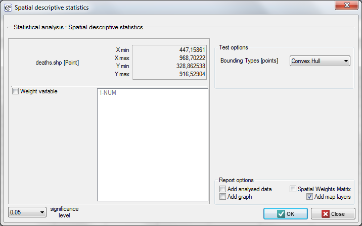
The window with settings for Descriptive statistics is accessed via the menu Spacial analysis \(\to\) Spatial descriptive statistics.
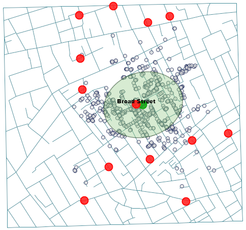
Example 1. (directory: snow, SHP files: deaths, pumps, streets) Data for the analysis are probably the best known, classical example of the use of cartography in epidemiology. They present the epidemic of cholera in London in 1854. The map which presents the range of the epidemic was made by John Snow, a doctor and the discoverer of the cause of the epidemic, considered to be one of the founders of epidemiology. The coordinates of points which constituted the basis for drawing the maps come from the original John Snow's map which was digitalized by Rusty Dodson from the US National Center for Geographic Information Analysis (http://ncgia.ucsb.edu/Publications/Software/cholera/) and later presented in meters.
After importing the above shapefiles (SHP) we can view and edit each of them in the Map manager.
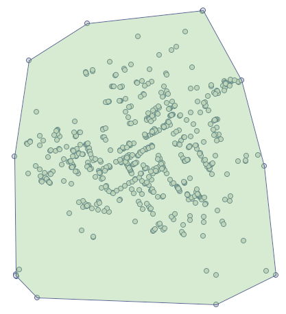
To conduct an analysis we select the deaths map and perform the Spatial descriptive statistics. Because we will utilize the map coordinates as data for the analysis, in the descriptive statistics window we select the option Use points from map coordinates and, as the bounding type, we select the Convex Hull.
 and selecting the layer of object bounding.
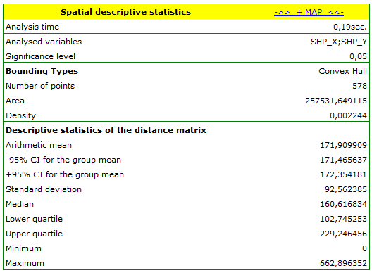
The analysis of the point distance matrix allows a more exact evaluation of their density. Some points are in the same place because the smallest distance is \(0m\). There are also points at a far greater distance from each other –the greatest distance is \(662.896352 m\). We can also find information about the average distance and the standard deviation of the points here.
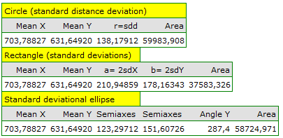
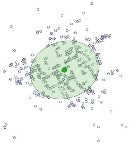
The most interesting information in the analysis of the deaths map is offered by the localized Center of point distribution (\(703.79\), \(631.65\)), together with the area of standard deviations which describe the the degree of concentration and the direction of dispersion (circle, ellipse, rectangle).
 .