 PQStat
As the number of variables subjected to a statistical analysis grows, the precision of the description of the phenomenon under study increases, but so does the level of complexity and the difficulty of interpreting the results obtained. Too large a number of variables carries the risk that some of them are correlated with one another, and therefore carry information that is partly repeated – already contained in other variables. The need to reduce the number of variables (dimensionality reduction) has given rise to a whole family of methods devoted to this issue, such as: factor analysis, principal component analysis, cluster analysis and discriminant analysis. These methods make it possible to detect relationships among variables and, on that basis, to distinguish groups of similar variables and select, for further analysis, either a single representative of each group, or a new variable whose values are computed from the remaining variables in the group. In this way we can be sure that the information carried by every group of variables is taken into account in the analysis – with only a small loss of information, a set of \(p\) variables can be reduced to a set of \(k\) variables, where \(k<p\).
Just as we may want to group variables, we may also want to group objects. Given information about certain characteristics of objects, we are often able to distinguish groups of objects that are similar with respect to these characteristics – for example, based on the amounts customers of a certain retail chain spend on particular products, customers can be divided into segments with similar purchasing preferences. As a result, an offer or advertisement can be prepared not for the general body of customers, but separately for each segment, so as to more precisely address the needs of a potential customer.
Principal component analysis
When to use:
Principal component analysis (PCA) is used to reduce the number of variables describing the objects under study. Instead of many, often mutually correlated, original variables, a small number of completely new variables – principal components – are computed, each being a linear combination of the original variables. Successive principal components are mutually uncorrelated (orthogonal), and their number (\(k\)) is less than or equal to the number of original variables (\(p\)).
A detailed principal component analysis makes it possible to identify which original variables have a strong influence on a given component, i.e. which together with it form a homogeneous group – the principal component then becomes the representative of that group. The new variables obtained in this way are usually fewer than the original variables, yet carry the same amount of information, or only slightly less. Moreover, because they are not correlated with one another, they can be successfully used in most subsequent multivariate analyses.
Assumptions
- the variables are measured on an interval scale,
- at least a few original variables are included in the analysis,
- the original variables are significantly correlated – if the variables are not correlated with one another (Pearson correlation coefficients close to 0), performing a principal component analysis makes no sense, since each variable would then already constitute a separate component; the degree of correlation among the variables can be assessed with Bartlett's test and the Kaiser-Meyer-Olkin (KMO) coefficient, both described below.
Definitions of measures
Each principal component is a linear combination of the original variables \(X_1,X_2,...,X_p\). Every component explains a certain part of the variability of the original variables and is therefore naturally based on measures of variability such as covariance (when the original variables are of similar size and expressed in the same units) or correlation (when the conditions needed to use covariance are not met). Each principal component is described by the following quantities.
- Eigenvalue
Indicates what part of the total variability of the original variables is explained by a given principal component. The first component explains the largest part of the variance, the second explains the largest part of the variance not explained by the first, and so on – each subsequent component explains the largest part of the variance not explained by the preceding components. As a result, each successive principal component explains a smaller and smaller part of the variance, i.e. the successive eigenvalues get smaller and smaller. Since the total variance is the sum of the eigenvalues, the percentage of variability explained by each component can be calculated, and, for successive components, the cumulative variability and the cumulative percentage of variability.- Eigenvector
Reflects the influence of the individual original variables on a given principal component – it contains the coefficients of the linear combination that defines the component. The sign of these coefficients indicates the direction of the influence and is arbitrary, which does not change the value of the information carried.- Factor loadings
Like the eigenvector, factor loadings reflect the influence of the individual original variables on a given principal component – they are values showing what part of the variance of a given component is accounted for by the original variables. When the analysis is based on the correlation matrix, these loadings are interpreted as correlation coefficients between the original variables and the given principal component.- Variable contributions
Based on the coefficients of determination between the original variables and a given principal component. They show what percentage of the variability of a given principal component can be explained by the variability of the individual original variables.- Communalities
Also based on the coefficients of determination between the original variables and a given principal component, but showing the reverse relationship – what percentage of the variability of a given original variable can be explained by the variability of the first several principal components. For example, the result for the second variable in the column for the fourth principal component tells us what percentage of the variability of the second variable can be explained by the variability of the first four principal components.
Graphical interpretation
Much of the information carried by the coefficients returned in the tables can be presented on a single chart. Such charts bring together, in one place, information about the mutual relationships among the components, the original variables and the cases, giving an overall picture of the analysis and providing a very good summary of it.
The factor loadings plot shows vectors, attached to the origin of the coordinate system, representing the original variables, placed on the plane defined by two selected principal components.
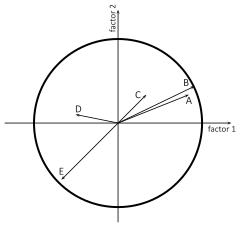
- The coordinates of the tip of the vector
are the corresponding factor loadings of the variable.
- The length of the vector
represents the amount of information about the original variable carried by the principal components that define the coordinate system – the longer the vector, the greater the contribution of the original variable to the components. In an analysis based on the correlation matrix, the loadings are correlations between the original variables and the components, so the points fall within the unit circle (a correlation coefficient cannot exceed one). The closer a given original variable lies to the edge of this circle, the better it is represented by the principal components shown.
- The sign of the coordinates of the tip of the vector
, i.e. the sign of the factor loading, indicates a positive or negative correlation between the original variable and the principal components forming the coordinate system. Considering both axes together (2 components), the original variables can be classified into one of four categories, depending on the combination of signs (\(+/-\)) of their factor loadings.
- The angle between vectors
indicates the correlation between the original variables:
\(0<\alpha<90^0\): the smaller the angle between the vectors representing the original variables, the stronger the positive correlation between these variables.
\(\alpha=90^0\) – the vectors are perpendicular, i.e. the original variables are not correlated.
\(90^0<\alpha<180^0\) – the larger the angle between the vectors representing the original variables, the stronger the negative correlation between these variables.
The biplot shows two series of data placed in the coordinate system defined by two principal components: the first series is the data from the factor loadings plot (the vectors of the original variables), and the second series consists of points representing the individual cases.
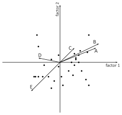
- The coordinates of the points
are interpreted like standardized values, i.e. positive coordinates indicate a value higher than the mean value of the principal component, negative ones indicate a lower value, and the higher the absolute value, the further the point lies from the mean. If atypical (outlying) observations appear on the plot, they may distort the analysis and should be removed, with the analysis then repeated.
- The distances between points
indicate the similarity of the cases – the closer two points lie to each other (in the sense of Euclidean distance), the more similar the information carried by the compared cases.
- The orthogonal projections of points onto the vectors
are interpreted in the same way as the coordinates of the points, except that they concern the original variables rather than the principal components. Values on the side of the tip of the vector are greater than the mean value of the original variable, while values on the extension of the vector in the opposite direction are smaller than the mean.
Criteria for dimensionality reduction
There is no single universal criterion for choosing the number of principal components, so it is good practice to be guided by several methods at once.
- Percentage of explained variance
All the principal components together carry 100% of the variance of the original variables. If the sum of the variances of the first few components accounts for a substantial part of the total variance, these components can satisfactorily replace the original variables. It is generally assumed that the selected principal components should account for over 80% of the variance.- Kaiser criterion
According to this criterion, only those principal components that have at least as much variance as any standardized original variable (i.e. variance equal to 1) are retained for interpretation. In other words, only components whose eigenvalue exceeds, or is close to, 1 are considered important.- Scree plot
Shows the rate at which the eigenvalues (the percentage of explained variance) decrease for successive components.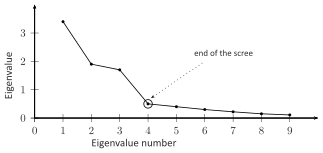
The point on the plot where this process stabilizes and the decreasing line becomes horizontal is the so-called end of the scree. The components to the right of this point represent negligible variance and, for the most part, represent random noise.
Computing the principal components
Once we have decided how many principal components we need, we can proceed to generate them. Principal components derived from the correlation matrix are computed as a linear combination of the standardized original variables, while those derived from the covariance matrix are computed as a linear combination of the original variables centred with respect to their mean.
Checking whether the analysis is warranted
Before proceeding to compute and interpret the principal components, it is worth checking whether the analysis makes sense at all, i.e. whether the original variables are sufficiently correlated with one another. Bartlett's test and the Kaiser-Meyer-Olkin (KMO) coefficient are used for this purpose.
- Bartlett's test
Tests the hypothesis that the correlation coefficients between the variables are zero (i.e. that the correlation matrix is the identity matrix). A statistically significant test result (\(p\) value lower than the assumed significance level \(\alpha\)) shows that the original variables are significantly correlated, and therefore that performing a principal component analysis makes sense.- Kaiser-Meyer-Olkin (KMO) coefficient
Assesses the degree of correlation among the original variables, i.e. the strength of the case for performing a principal component analysis. The coefficient's value lies in the range \(<0,1>\) – low values indicate that there is no basis for performing the analysis, while high values are a reason to perform it.
How to set up the analysis
The window with the settings for Principal component analysis is opened via the menu Statistics \(\to\) Multivariate models \(\to\) Principal component analysis.
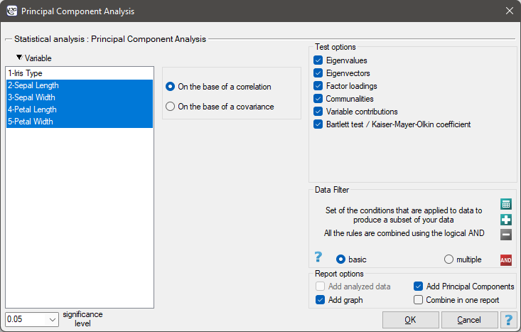
Performing and interpreting the analysis
Example 1. (file: iris.pqs)
This classic data set was originally published in R.A. Fisher's 1936 paper[60], which introduced discriminant analysis. The file contains measurements (in centimetres) of the length and width of the petals and sepals for 3 varieties of iris. The species studied are setosa, versicolor and virginica. It is of interest to determine how these species can be distinguished on the basis of the measurements obtained.
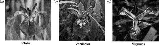
The figure comes from Lee et al. (2006): "Application of a noisy data classification technique to determine the occurrence of flashover in compartment fires"
Principal component analysis will let us identify which measurements (the length and width of the petals and sepals) give the researcher the most information about the observed flowers.
The first step, carried out even before computing and analysing the components, is to check whether performing this analysis is worthwhile. We therefore start by computing the correlation matrix of the variables and examining the correlations obtained using Bartlett's test and the KMO coefficient.
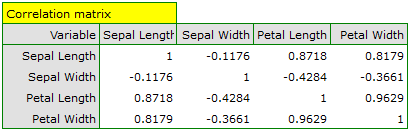
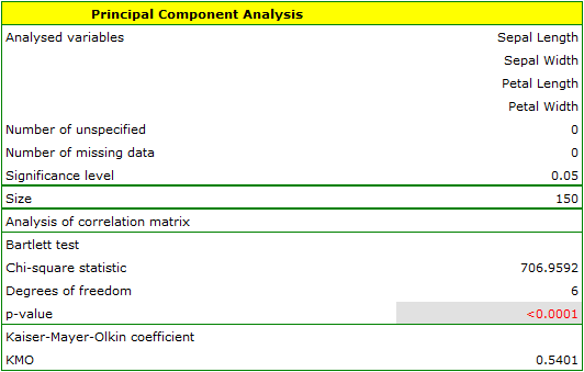
The first result of this analysis that deserves special attention is the eigenvalues:
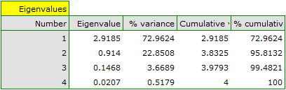
The eigenvalues obtained show that two, or even a single, principal component will describe our data well. The eigenvalue for the first component is 2.92, and the percentage of variance it explains is 72.96%. The second component explains considerably less variance, 22.85%, and its eigenvalue is 0.91. According to the Kaiser criterion, only a single principal component is sufficient for interpretation, since only the first component has an eigenvalue greater than 1. Looking at the scree plot, however, we can conclude that the decreasing line only becomes horizontal from the third principal component onward.
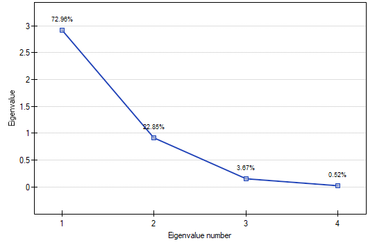
In line with this, the first two components carry significant information – together they explain as much as 95.81% of the variance (see the cumulative % column).
The communalities for the first component are high for all the original variables except sepal width, for which it is 21.17%. This means that if we were to rely only on the first component, the variable sepal width would be poorly represented.
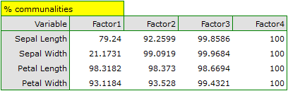
For the first two components, the communalities are already at a similarly very high level – for every variable analysed they exceed 90%, i.e. the variance of each variable is represented by these two components to a degree of over 90%. Having gathered all this information, it was decided to extract and interpret 2 components.
To take a closer look at the relationship between the principal components and the original variables, i.e. the length and width of the petals and sepals, we interpret: the eigenvectors, the factor loadings and the variable contributions.
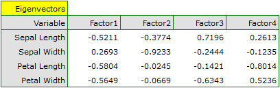
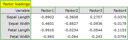
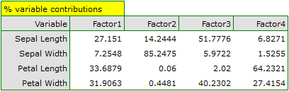
The individual original variables affect the first principal component to different degrees. Let us rank them by the size of this influence:
- Petal length is negatively correlated with the first component, so the longer the petal, the lower the value of this component. The eigenvector for petal length is the largest in this component, at \(-0.58\). Its factor loading tells us that the correlation between the first principal component and petal length is very high, at \(-0.99\), giving a 33.69% contribution to the first component;
- Petal width has only a slightly smaller influence on the first component and is also negatively correlated with it;
- Sepal length is interpreted similarly to the two previous variables, but its influence on the first component is smaller;
- Sepal width is the most weakly correlated with the first component, and the sign of this correlation is positive.
The second component mainly represents the original variable sepal width – the remaining original variables are only weakly reflected in it. The eigenvector, factor loading and contribution of sepal width are the highest of all the variables in the second component.
Each principal component defines a homogeneous group of original variables. We will call the first component "petal size", since the variables that matter most for it are those carrying information about the petal, although it should be noted that sepal length also has a considerable influence on the value of this component. In interpreting it, we should remember that the larger the values of this component, the smaller the petals. We will call the second component "sepal width", since only sepal width is reflected in it to any great extent. The larger the values of this component, the narrower the sepal.
Finally, we generate the components by selecting the option Add principal components in the analysis window. An excerpt of the result obtained is shown below:
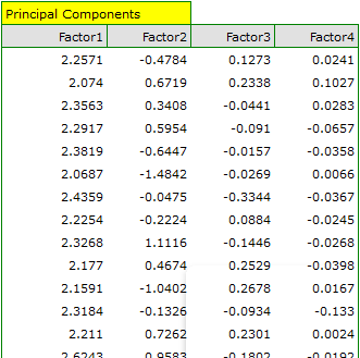
So that the first two components can be used instead of the four original variables, we finally paste them into the data sheet. The researcher can now carry out any further planned statistics on two new, uncorrelated variables.
- Analysis of the plots of the first two components
Analysing the plots not only leads the researcher to the same conclusions as analysing the tables, but also makes it possible to assess the results obtained more thoroughly.- Factor loadings plot
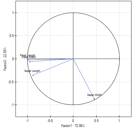
The plot shows the first two principal components, which represent 72.96% and 22.85% of the variance, giving a combined total of 95.81% of the variance of the original variables.
The vectors representing the original variables almost reach the edge of the unit circle (a circle of radius 1), so all of them are very well represented by the first two principal components forming the coordinate system.
The angle between the vectors depicting petal length, petal width and sepal length is small, meaning these variables are strongly correlated. The correlation of these variables with the components forming the coordinate system is negative – the vectors lie in the third quadrant of the plot, with higher coordinate values for the tip of the vector observed for the first component than for the second. Such an arrangement of vectors indicates that they form a homogeneous group, represented mainly by the first component.
The vector for sepal width points in an entirely different direction; it is only weakly correlated with the remaining original variables, as shown by its angle to them, which is close to a right angle. Its correlation with the first component is positive but not very high (a low value of the first coordinate of the tip of the vector), while its correlation with the second component is negative and high (a high value of the second coordinate of the tip of the vector). We conclude from this that sepal width is the only original variable that is well represented by the second component.- Biplot
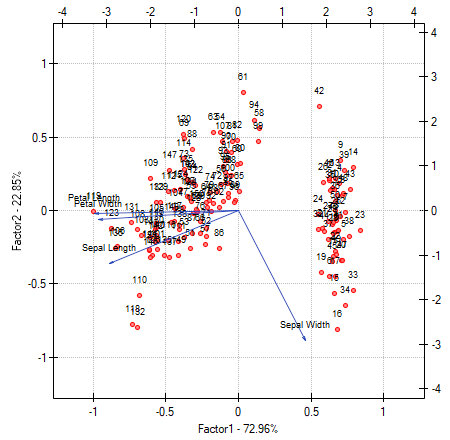
The biplot shows two series of data plotted against the first two components. One series consists of the vectors of the original variables, already shown in the previous plot, and the other consists of points carrying information about the individual flowers, with the values of the second series read from the upper \(X\) axis and the right-hand \(Y\) axis. The interpretation of the vectors, i.e. the first series, was discussed for the previous plot. To understand how to interpret the points, let us focus on the flowers numbered 33 and 34, and on flower number 109.
Flowers 33 and 34 are similar to each other – the distance between them is small. Both points have a value of the first component considerably higher than average, and a value of the second component considerably lower than average. The average value, i.e. the arithmetic mean of both components, is 0, so this is the centre of the coordinate system. Recalling that the first component mainly represents petal size and the second mainly represents sepal width, we can say that flowers 33 and 34 have small petals and wide sepals. Flower 109, on the other hand, is a point located far away from the other two. It has a negative first component and a positive, but not high, second component, i.e. it is a flower with relatively large petals and a sepal width only slightly smaller than average.
Similar information can be obtained by projecting the points onto the lines extending the vectors of the original variables. For example, flower 33 has a large sepal width (high, positive projection values onto the original variable sepal width), but low values of the remaining original variables (negative projection values onto the extensions of the vectors depicting the remaining original variables).
Formulas:
Each principal component is a linear combination of the original variables:
where:
\(X_1,X_2,...,X_p\) – the original variables,
\(a_{i1}, a_{i2},...,a_{ip}\) – the coefficients of the \(i\)th principal component.
The mathematical computations needed to extract the principal components amount to finding the eigenvalues and the corresponding eigenvectors from the matrix equation:
where:
\(\lambda\) – the eigenvalues,
\(a_i=(a_{i1}, a_{i2},...,a_{ip})\) – the eigenvector corresponding to the \(i\)th eigenvalue,
\(M\) – the variance or covariance matrix of the original variables \(X_1,X_2,...,X_p\),
\(I\) – the identity matrix (1 on the main diagonal, 0 elsewhere).
The percentage of variability explained by the \(i\)th principal component is given by the formula:
Bartlett's test
Hypotheses:
\(\begin{array}{cl} \mathcal{H}_0: & M = I, \\ \mathcal{H}_1: & M \ne I. \end{array}\)
where:
\(M\) – the variance or covariance matrix of the original variables \(X_1,X_2,...,X_p\),
\(I\) – the identity matrix (1 on the main diagonal, 0 elsewhere).
Formulas:
The test statistic is given by:
where:
\(p\) – the number of original variables,
\(n\) – the sample size (number of cases),
\(\lambda_i\) – the \(i\)th eigenvalue.
This statistic asymptotically (for large expected frequencies) has the \(\chi^2\) distribution with \(p(p-1)/2\) degrees of freedom.
The \(p\) value, determined on the basis of the test statistic, is compared with the significance level \(\alpha\):
The Kaiser-Meyer-Olkin coefficient – formula:
where:
\(r_{ij}\) – the correlation coefficient between the \(i\)th and \(j\)th variable,
\(\hat{r}_{ij}\) – the partial correlation coefficient between the \(i\)th and \(j\)th variable.