The t-test for dependent groups

When to use this test:

The \(t\)-test for dependent groups is used when the same characteristic is measured twice for the same subjects, under different conditions (e.g. before and after a diet), and we want to check whether the measurement changed.

Assumptions

measurement on an interval scale,
normality of distribution of the differences \(d_i\),
a dependent model.

How to set up the analysis

Statistics \(\to\) Parametric tests \(\to\) \(t\)-test for dependent groups (or via the Wizard).

Step 1. Indicate the two variables corresponding to the first and second measurement (e.g. BMI before the diet and BMI after the diet).

Step 2. Run the analysis.

Note! Calculations can be based on raw data or on averaged data, i.e. the mean of the differences, the standard deviation of the differences, and the sample size.

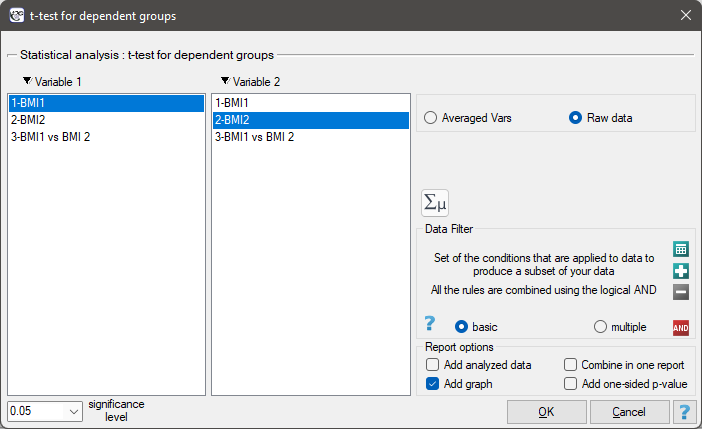
Performing and interpreting the analysis

Example 1. (BMI.pqs file)
A clinic treating eating disorders studied the effect of a recommended "diet A" on body weight change. A sample of 120 obese patients were put on the diet. Their BMI levels were measured twice: before the diet and after 180 days of following it. The aim of the study was to compare the obtained BMI measurements in order to assess the effectiveness of the diet.

The distribution of the difference between the pairs of measurements was a normal distribution (Lilliefors test, \(p=0.0837\)), which allowed the \(t\)-test for dependent groups to be applied.

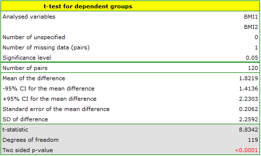
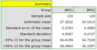
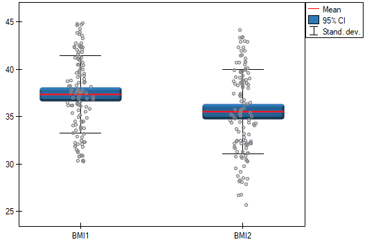
\(p<0.0001\) (statistically significant, \(\alpha=0.05\))

The mean BMI of the studied patients changed significantly under the influence of the diet – before the diet it was higher on average by less than 2 units.

The \(p\) value, calculated on the basis of the test statistic, is always compared with the assumed significance level \(\alpha\): when \(p \le \alpha\), the change is statistically significant; when \(p > \alpha\), there is no reason to claim that a change occurred. It is also worth reporting the effect size (Cohen's d) – statistical significance alone does not indicate how large the change is; with large samples, even small differences may turn out to be statistically significant.

Definitions of measures

Cohen's d – a standardized effect-size measure that determines how large a part of the observed variability in the data is the observed difference between the means. Unlike the \(p\) value, it does not depend on sample size, which makes it possible to assess the practical significance of a difference, not just its statistical significance.

FOR THOSE INTERESTED

Hypotheses:

\(\begin{array}{cc} \mathcal{H}_0: & \mu_0=0,\\ \mathcal{H}_1: & \mu_0\ne0, \end{array}\)

where \(\mu_0\) – mean of the differences \(d_i\) in the population.

Formulas:

The test statistic is defined by:

\[ t=\frac{\overline{d}}{sd_d}\sqrt{n}, \]

where \(\overline{d}\) – mean of the differences \(d_i\) in the sample, \(sd_d\) – standard deviation of the differences \(d_i\) in the sample, \(n\) – number of differences \(d_i\) in the sample. The test statistic has the \(t\)-Student distribution with \(n-1\) degrees of freedom.

Standard deviation of the difference:

\[ sd_d=\displaystyle{\sqrt{\frac{\sum_{i=1}^{n}(d_i-\overline{d})^2}{n-1}}}, \]

Standard error of the mean of differences:

\[ SEM_{d}=\displaystyle{\frac{SD_d}{\sqrt{n}}}. \]

Cohen's d formula:

Cohen's d is calculated using the formula:

\[ d=\left|\frac{\overline{d}}{sd_d}\right| \]

When interpreting an effect, researchers often use general guidelines proposed by Cohen [47] defining small (0.2), medium (0.5) and large (0.8) effect sizes.