 PQStat
Tests for one proportion
When to use this test:
Tests for one proportion are used when there are two possible outcomes to obtain (one of which is a distinguished outcome, with count \(m\)), and we know how often these outcomes occur in the sample (we know the proportion \(p\)). These tests are used to verify the hypothesis that the proportion in the population from which the sample is drawn is a given value. Depending on the sample size \(n\), we can choose between the \(Z\) test for one proportion – for large samples, and the exact binomial test – for small samples.
Assumptions
- measurement on a nominal scale – any ordering of the categories is not taken into account.
Definitions of measures
Confidence interval for a proportion – for the sample estimator, which in this case is the proportion value \(p\), a confidence interval is calculated. For large samples, one can rely on intervals based on the normal distribution – the so-called Wald intervals. More universal, however, are the intervals proposed by Wilson (1927)[177], as well as by Agresti and Coull (1998)[5]. The Clopper-Pearson intervals (1934)[40] are more accurate for smaller samples. A comparison of methods for constructing confidence intervals for proportions can be found in the work of Brown L.D. and others (2001)[31].
How to set up the analysis
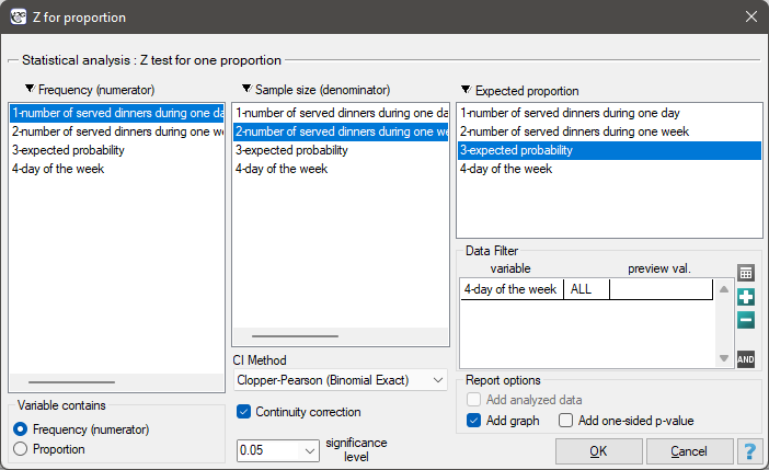
Statistics \(\to\) Nonparametric tests \(\to\) Z for proportion.
Performing and interpreting the analysis
Continuation of Example 1 (dinners.pqs file): suppose we would like to check whether \(\frac{1}{5}\) of all the dinners served in the school canteen over the week are served on Friday. For the sample drawn, \(m=20\), \(n=150\).

When setting the analysis options, we enable a filter, selecting the appropriate day of the week – Friday. Not setting the filter does not generate an error, but simply results in statistics being calculated for each successive day of the week.
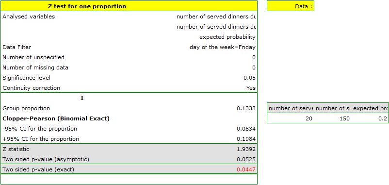
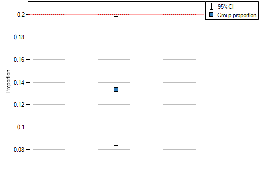
The proportion of the distinguished value in the sample is \(p=\frac{m}{n}=0.133\), and the 95% Clopper-Pearson confidence interval for this fraction, \((0.083, 0.198)\), does not include the hypothetical value of 0.2.
Hypotheses:
\( \begin{array}{cl} \mathcal{H}_0: & p=p_0,\\ \mathcal{H}_1: & p\neq p_0, \end{array} \)
where:
\(p\) – the probability (distinguished proportion) in the population,
\(p_0\) – the expected probability (expected proportion).
The \(Z\) test for one proportion (\(Z\) test for one proportion)
Formulas: The test statistic is defined by:
where:
\(p=\frac{m}{n}\) – the proportion for the sample from this population,
\(m\) – the count of the distinguished values in the sample,
\(n\) – the sample size.
The test statistic modified with the continuity correction is defined by:
The \(Z\) statistic, both without and with this correction, asymptotically (for large sample sizes) has the normal distribution.
The binomial test (Binomial test for one proportion)
Definition: This test directly uses the binomial distribution, also called the Bernoulli distribution, which belongs to the group of discrete distributions (i.e. distributions in which the analysed variable takes a finite number of values). The analysed variable can take \(k=2\) values, the first usually referred to as a success and the second as a failure. The probability of a success is \(p_0\), and of a failure \(1-p_0\).
Formulas: The probability for a specific point in this distribution is calculated using the formula:
where:
\({n \choose m}=\frac{n!}{m!(n-m)!}\),
\(m\) – the count of the distinguished values in the sample,
\(n\) – the sample size.
Interpretation: On the basis of the sum of the appropriate probabilities \(P\), a one-sided and a two-sided \(p\) value are determined, with the two-sided \(p\) value defined as twice the smaller of the one-sided probabilities. The \(p\) value is compared with the significance level \(\alpha\): if \(p \le \alpha\), we reject \(\mathcal{H}_0\) in favor of \(\mathcal{H}_1\); if \(p > \alpha\), there is no reason to reject \(\mathcal{H}_0\).