The Chi-square test for trend

When to use this test:

The \(\chi^2\) test for trend, also called the Cochran-Armitage trend test (ang. Cochran-Armitage test for trend)[43][10], is used when we have ordered categories of one feature (e.g. education level) and two groups of the other feature (e.g. smoker/non-smoker), and we want to check whether the proportions across the ordered categories increase or decrease in a systematic way – i.e. whether a trend is visible.

Assumptions

measurement on an ordinal scale or an interval scale (the categories must be orderable),
an independent model (the second feature – 2 independent groups).

How to set up the analysis

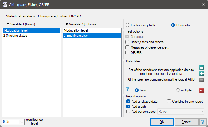
Statistics \(\to\) NonParametric tests \(\to\) Chi-square, Fisher, OR/RR, option Fisher, Yates and others... \(\to\) Chi-square for trend.

Step 1. Indicate the ordered feature (e.g. education) and the two-category feature (e.g. smoking).

Step 2. Run the analysis.

Note! Before the analysis, you need to indicate the order in which the categories of the ordered feature should appear. To do this, from the variable's properties select Codes/Labels/Format... and assign the order by specifying consecutive natural numbers, then assign labels to them.

Performance and interpretation

Example 1. (smoking-education.pqs file)
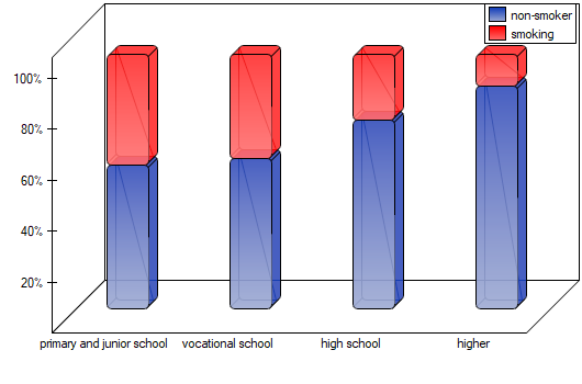
We check whether cigarette smoking is related to the education of residents of a village. A sample of 122 people was drawn. We assume that the relationship can be of two types: the more educated people are, the more often they smoke, or the more educated people are, the less often they smoke – so we are looking for an increasing or decreasing trend.

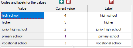
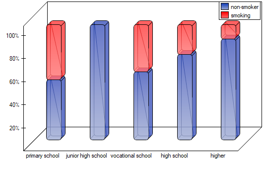
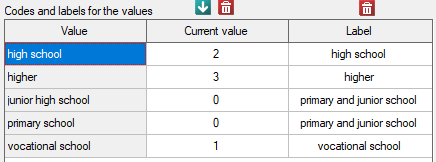
\(p=0.0091\) (statistically significant, \(\alpha=0.05\))

There is a trend in the frequency of smoking with increasing education in the analysed population.

As the graph shows, the more educated people are, the less often they smoke. However, the result obtained for people with lower secondary education deviates from this trend – since this category has only two people, it did not have much effect on the overall trend. Due to the very small size of this group, the analysis was repeated for the combined primary and lower secondary education categories.

\(p=0.0078\) (after combining categories, statistically significant, \(\alpha=0.05\))

The trend in smoking frequency with increasing education is confirmed again after combining the least numerous categories.

Example 2. (viewers.pqs file)
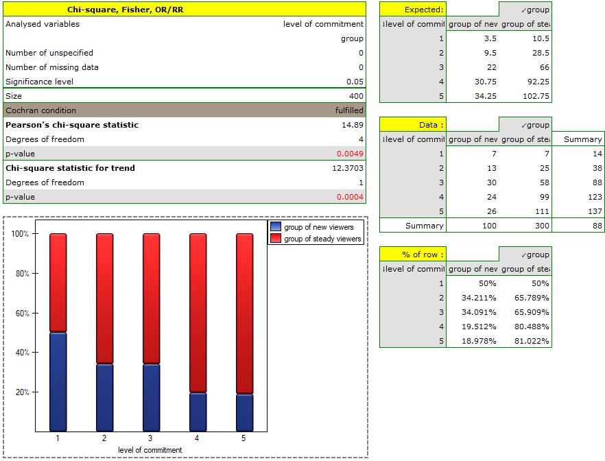
Because of a decrease in the audience of a particular soap opera, a viewer opinion survey was carried out. 100 people who had recently started watching the soap opera and 300 who had watched it regularly from the beginning were surveyed. Among other things, they were asked to rate their level of preoccupation with the characters' fate. The results are shown in the table below:

Level of	group
commitment	group of new viewers	group of steady viewers	total
rather small	7	7	14
average	13	25	38
rather high	30	58	88
high	24	99	123
very high	26	111	137
total	100	300	400

The new viewers make up 25% of all analysed viewers. This proportion is not the same for every level of commitment, however – it looks as follows:

Level of	group
commitment	group of new viewers	group of steady viewers	total
rather small	\(p_1\)=50.00%	50.00%	100%
average	\(p_2\)=34.21%	65.79%	100%
rather high	\(p_3\)=34.09%	65.91%	100%
high	\(p_4\)=19.51%	80.49%	100%
very high	\(p_5\)=18.98%	81.02%	100%
total	25.00%	75.00%	100%

\(p=0.000436\) (statistically significant, \(\alpha=0.05\))

There is a trend in the proportion of new viewers in the population of soap opera viewers: the more interested a group is in the characters' fate, the smaller share of it is made up of new viewers (a decreasing trend).

FOR THOSE INTERESTED

Notation: the \(r\times 2\) contingency table of observed frequencies:

Observed frequencies		Feature 2 (group)
\(O_{ij}\)		\(G_1\)	\(G_2\)	Total
Feature 1 (feature \(X\))	\(X_1\)	\(O_{11}\)	\(O_{12}\)	\(W_1=O_{11}+O_{12}\)
	\(X_2\)	\(O_{21}\)	\(O_{22}\)	\(W_2=O_{21}+O_{22}\)
	...	...	...	...
	\(X_r\)	\(O_{r1}\)	\(O_{r2}\)	\(W_r=O_{r1}+O_{r2}\)
	Total	\(C_1=\sum_{i=1}^rO_{i1}\)	\(C_2=\sum_{i=1}^rO_{i2}\)	\(n=C_1+C_2\)

Let \(p_1, p_2, ..., p_r\) denote the proportions \(p_1=\frac{O_{11}}{W_1}\), \(p_2=\frac{O_{21}}{W_2}\),..., \(p_r=\frac{O_{r1}}{W_r}\).

Hypotheses:

\[\begin{array}{cl} \mathcal{H}_0: & \text{in the analysed population, there is no trend in the proportions }p_1, p_2, ..., p_r\text{, }\\ \mathcal{H}_1: & \text{in the analysed population, there is a trend in the proportions }p_1, p_2, ..., p_r\text{. } \end{array}\]

Formulas: The test statistic is defined by:

\[ \chi^2=\frac{\left[\left(\sum_{i=1}^r i\cdot O_{i1}\right) -C_1\left(\sum_{i=1}^r\frac{i\cdot W_i}{n}\right)\right]^2}{\frac{C_1}{n}\left(1-\frac{C_1}{n}\right)\left[\left(\sum_{i=1}^n i^2 W_i\right)-n\left(\sum_{i=1}^n\frac{i \cdot W_i}{n}\right)^2\right]}. \]

This statistic has the \(\chi^2\) distribution with 1 degree of freedom.