 PQStat
The single-sample chi-square test for a population variance
When to use this test:
The \(\chi^2\) test for the variance of a single sample (The Single-Sample Chi-square Test for a Population Variance) lets you verify the hypothesis that the sample studied comes from a population for which the variance (or standard deviation \(\sigma\)) is a given value. Hypotheses can refer either to the variance or, equivalently, to the standard deviation.
Assumptions
- measurement on an interval scale,
- normality of distribution of the feature studied.
How to set up the analysis
Statistics \(\to\) Parametric tests \(\to\) Chi-square test for variance.
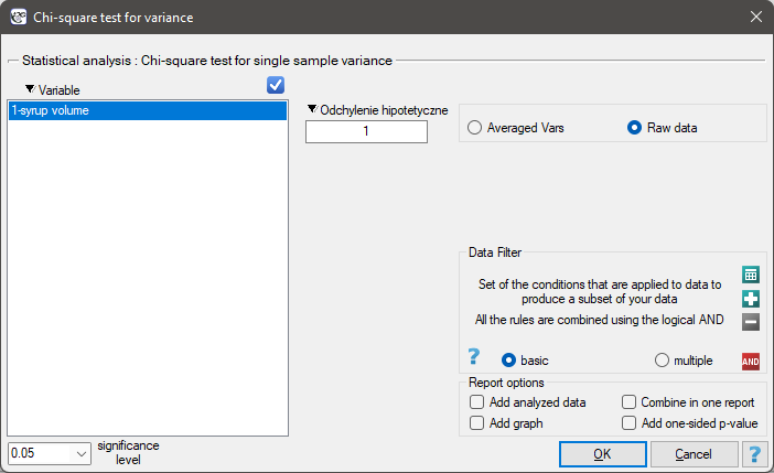
Performing and interpreting the analysis
Example 1. (dispenser.pqs file)
Before starting production of another batch of a certain cough syrup, control measurements were made of the volume of syrup poured into bottles. The technical documentation of the dosing device shows that the permissible variation in syrup volume, measured by the standard deviation, is 1 ml. We need to check whether the tested device is working properly.
The normality of the distribution of the volume of syrup poured into bottles was checked (with the Lilliefors test), obtaining a result consistent with this normality. The analysis concerning the standard deviation can therefore be performed with the chi-square test for variance.
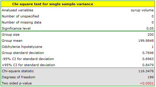
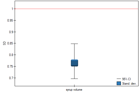
We can, however, consider the device's performance to be correct, because the sample standard deviation is 0.76, which is significantly smaller than the permissible value from the technical documentation.
Hypotheses:
\(\begin{array}{cc} \mathcal{H}_0: & \sigma=\sigma_0,\\ \mathcal{H}_1: & \sigma\ne \sigma_0, \end{array}\)
where:
\(\sigma\) – the standard deviation of the feature in the population represented by the sample,
\(\sigma_0\) – a given value.
Formulas: The test statistic is defined by:
where:
\(sd\) – the sample standard deviation,
\(n\) – the sample size.
Interpretation: The test statistic has the \(\chi^2\) distribution with the number of degrees of freedom calculated using the formula \(df=n-1\).
The \(p\) value, determined on the basis of the test statistic and the \(\chi^2\) distribution, is compared with the significance level \(\alpha\): if \(p \le \alpha\), we reject \(\mathcal{H}_0\) in favor of \(\mathcal{H}_1\); if \(p > \alpha\), there is no reason to reject \(\mathcal{H}_0\).
If the standard deviation value is smaller than the given value, the \(p\) value is calculated as twice the area under the chi-square distribution curve to the left of the corresponding critical value; if it is larger than the given value, it is twice the corresponding area to the right.