 PQStat
The linear correlation coefficients
When to use:
The Pearson product-moment correlation coefficient \(r_p\) (Pearson (1896, 1900)) is used to examine the strength of the linear relationship between two features.
Assumptions
- measurement on an interval scale,
- no outliers,
- normality of distribution of the analysed features or normality of the model residuals.
Definitions of measures
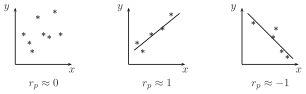
The Pearson product-moment correlation coefficient \(r_p\) – describes the strength and direction of the linear relationship between two interval features. The value \(r_p\in\langle-1;1\rangle\) is interpreted as follows:
- \(r_p\approx1\) means a strong positive linear relationship, i.e. the measurement points lie close to a straight line, and an increase in the independent variable corresponds to an increase in the dependent variable;
- \(r_p\approx-1\) means a strong negative linear relationship, i.e. the measurement points lie close to a straight line, but an increase in the independent variable corresponds to a decrease in the dependent variable;
- when the coefficient is equal or very close to zero, there is no linear relationship between the analysed features (a non-linear relationship may still exist).
Chart 1. Graphical interpretation of the \(r_p\) coefficient.
When one of the two analysed features is constant (regardless of changes in the other feature), the two features are not related, and the \(r_p\) coefficient cannot be calculated.
The coefficient of determination \(r_p^2\) – expresses the percentage of variability in the dependent variable explained by variability in the independent variable.
The resulting correlation model represents a linear relationship of the form:
where the coefficients \(\beta\) and \(\alpha\) of the linear regression equation are the slope and the intercept of the regression line.
Formulas:
where:
\(x_i, y_i\) – successive values of feature \(X\) and \(Y\),
\(\overline{x}, \overline{y}\) – means of the values of feature \(X\) and feature \(Y\),
\(n\) – sample size.
\(R_p\) denotes the Pearson correlation coefficient in the population, while \(r_p\) denotes it in the sample.
The coefficients of the linear regression equation are calculated using the formulas:
The Pearson correlation coefficient significance
When to use this test:
The test of significance for the Pearson product-moment correlation coefficient lets you check whether a linear relationship exists between the analysed features of a population. It is based on the Pearson product-moment correlation coefficient \(r_p\) calculated for the sample – the closer the value of \(r_p\) is to 0, the weaker the relationship joining the analysed features.
Assumptions
- measurement on an interval scale,
- normality of distribution of the analysed features in the population, or normality of the model residuals.
How to set up the analysis
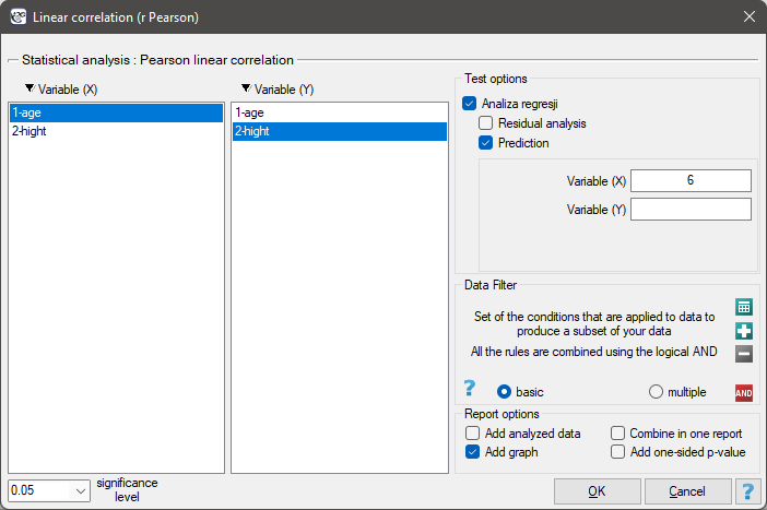
Statistics \(\to\) Parametric tests \(\to\) linear correlation (r-Pearson) (or via the Wizard).
Performing and interpreting the analysis
Example 1. (age-height.pqs file)
Among the students of a certain ballet school, the relationship between age and height was studied. A sample of sixteen children was drawn, and the following measurements of these features were recorded:
(age, height): (5, 128) (5, 129) (5, 135) (6, 132) (6, 137) (6, 140) (7, 148) (7, 150) (8, 135) (8, 142) (8, 151) (9, 138) (9, 153) (10, 159) (10, 160) (10, 162).
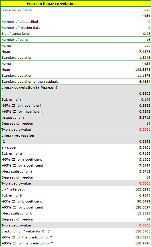
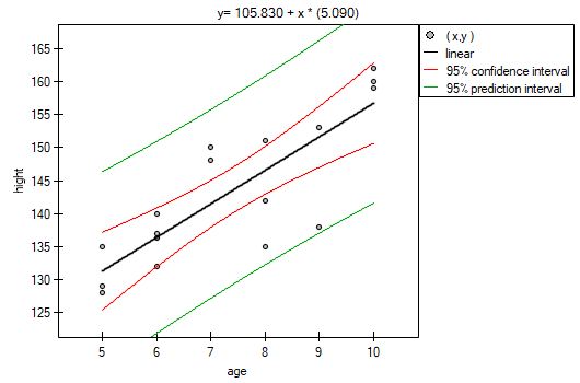
This relationship is directly proportional, meaning that as the children's age increases, so does their height. The Pearson product-moment correlation coefficient, and thus the strength of the linear relationship between age and height, is \(r_p=0.8302\). The coefficient of determination \(r_p^2=0.6892\) means that about 69% of the variability in height is explained by the variability in age.
From the regression equation:
we can calculate a predicted value for a child aged, for example, 6 years. The predicted height of such a child is 136.37 cm.
Hypotheses:
\(\begin{array}{cl} \mathcal{H}_0: & R_p = 0, \\ \mathcal{H}_1: & R_p \ne 0. \end{array}\)
Formulas:
The test statistic is defined by:
where \(\displaystyle SE=\sqrt{\frac{1-r_p^2}{n-2}}\).
The value of the test statistic cannot be calculated when \(r_p=1\) or \(r_p=-1\), or when \(n<3\). The test statistic has the \(t\)-Student distribution with \(n-2\) degrees of freedom.
The \(p\) value, determined on the basis of the test statistic, is compared with the significance level \(\alpha\): if \(p \le \alpha\), we reject \(\mathcal{H}_0\) in favor of \(\mathcal{H}_1\); if \(p > \alpha\), there is no reason to reject \(\mathcal{H}_0\).
The slope coefficient significance
When to use this test:
The \(t\)-test for the significance of the coefficients of the linear regression equation lets you check whether a linear relationship exists between the analysed features of a population, based on the slope coefficient \(\beta\) calculated for the sample – the closer the value of \(\beta\) is to 0, the weaker a relationship the fitted line represents. In a regression with a single independent variable, this test is equivalent to the test of significance for the Pearson correlation coefficient – it gives exactly the same \(p\) value.
Assumptions
- measurement on an interval scale,
- normality of distribution of the analysed features in the population, or normality of the model residuals.
Performing and interpreting the analysis
Because of its equivalence to the test of significance for the Pearson correlation coefficient with a single independent variable, the performance and interpretation of this test coincide with Example 1 above.
Analysis of model residuals – explained in the Multiple Linear Regression module.
Hypotheses:
\(\begin{array}{cl} \mathcal{H}_0: & \beta = 0, \\ \mathcal{H}_1: & \beta \ne 0. \end{array}\)
Formulas:
The test statistic is defined by:
where:
\(\displaystyle SE=\frac{s_{yx}}{sd_x\sqrt{n-1}}\),
\(s_{yx}=sd_y \sqrt{\frac{n-1}{n-2}(1-r^2)}\),
\(sd_x, sd_y\) – standard deviation of the values of feature \(X\) and feature \(Y\).
The value of the test statistic cannot be calculated when \(r_p=1\) or \(r_p=-1\), or when \(n<3\). The test statistic has the \(t\)-Student distribution with \(n-2\) degrees of freedom.
The \(p\) value, determined on the basis of the test statistic, is compared with the significance level \(\alpha\): if \(p \le \alpha\), we reject \(\mathcal{H}_0\) in favor of \(\mathcal{H}_1\); if \(p > \alpha\), there is no reason to reject \(\mathcal{H}_0\).
Prediction
When to use:
Prediction consists in predicting the value of one variable (most often the dependent variable \(y_0\)) on the basis of the value of another variable (most often the independent variable \(x_0\)), using the calculated linear regression equation. The accuracy of the predicted value is expressed by the prediction intervals calculated for it.
Definitions of measures
Interpolation – consists in predicting the value of a given variable that lies inside the range for which the regression model was built. Interpolation is generally a safe procedure – it only assumes continuity of the function expressing the relationship between the two variables.
Extrapolation – consists in predicting the value of a given variable that lies outside the range for which the regression model was built. Unlike interpolation, extrapolation is often a risky procedure and is only performed a short distance from the range for which the regression model was built.
How to set up the analysis
In the Pearson linear correlation analysis window, select the Prediction button and indicate the values of the independent variable for which you want to carry out the prediction.
Performing and interpreting the analysis
See Example 1 above – the predicted height of a 6-year-old child, calculated from the regression equation, is exactly the result of such a prediction (interpolation, since age 6 falls within the range of the data on which the model was built).