 PQStat
The Cohen's Kappa coefficient and a test to examine its significance
When to use:
The Cohen's Kappa coefficient (Cohen J., 1960[45]) determines the degree of agreement between two measurements of the same variable made under different conditions. The same variable may be measured by two different raters (reproducibility), or by one rater twice (repeatability). The \(\hat \kappa\) coefficient is calculated for dependent categorical variables, on the basis of raw data or a \(c\times c\) contingency table built from it.
Assumptions
- measurement on a nominal scale (unweighted Kappa, i.e. Cohen's Kappa) or an ordinal scale (weighted Kappa).
Definitions of measures
The Kappa coefficient (\(\hat \kappa\)) – its value lies in the range from \(-1\) to \(1\). A value of 1 means full agreement, a value of 0 means agreement at the same level that would arise from a random distribution of the data in a contingency table. The range between 0 and \(-1\) is practically never used – a negative \(\hat \kappa\) value means agreement at a level lower than would arise from a random distribution of the data in the contingency table. \(\hat \kappa\) denotes the agreement coefficient in the sample, while \(\kappa\) denotes it in the population.
Depending on requirements, unweighted Kappa (i.e. Cohen's Kappa) or weighted Kappa can be determined. The assigned weights (\(w_{ij}\)) refer to the individual cells of the contingency table: on the diagonal they equal 1, and off the diagonal they lie in the range \(\langle0;1)\).
Unweighted Kappa – calculated for data whose categories cannot be ordered, e.g. data comes from patients divided by the type of disease diagnosed, and these diseases cannot be ordered (pneumonia (1), bronchitis (2), other (3)). In such a situation, the agreement of diagnoses made by two doctors can be checked using unweighted Kappa, i.e. Cohen's Kappa. The disagreement of pairs \(\{(1),(3)\}\) and \(\{(1),(2)\}\) is treated equivalently, so the off-diagonal weights of the weight matrix are set to zero.
Weighted Kappa – in a situation where the data categories can be sorted (e.g. data comes from patients divided by the degree of lesion severity into: no lesion (1), mild lesion (2), suspected cancer (3), cancer (4)), the agreement of ratings given by two radiologists can be built while taking into account the possibility of sorting. The pair of ratings \(\{(1),(4)\}\) may then be considered more discordant than \(\{(1),(2)\}\). For the order of the categories to affect the agreement result in this way, weighted Kappa should be determined. The assigned weights can take a linear or quadratic form (Cicchetti, 1971[38]; Cohen, 1968[46]) – the further from the diagonal of the matrix, the smaller the weight, with linear weights decreasing proportionally, and quadratic weights decreasing more slowly closer to the diagonal and more rapidly further away. Quadratic weights are of greater interest because of the practical interpretation of the Kappa coefficient, which in that case is identical to the intraclass correlation coefficient[62].
How to set up the analysis
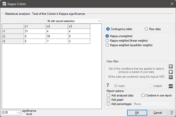
Statistics \(\to\) Nonparametric tests \(\to\) Kappa-Cohen (or via the Wizard).
Performing and interpreting the analysis
Example 1. (diagnosis.pqs file)
We examine the agreement of the diagnosis made by 2 doctors. To do this, we draw a sample of 110 patients from a children's hospital. The doctors see patients in neighbouring consulting rooms. Each patient is examined first by doctor A and then by doctor B. The diagnoses made by the doctors are shown in the table below.
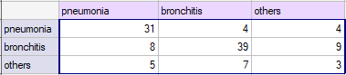
We could examine the agreement of the diagnosis using the plain percentage of concordant values. In our example, the doctors gave a concordant diagnosis for 73 patients (31+39+3=73), which is 66.36% of the group studied. The Kappa coefficient adjusts this value for the chance of agreement (i.e. it corrects for the agreement that arises from a random distribution of the data in the table).
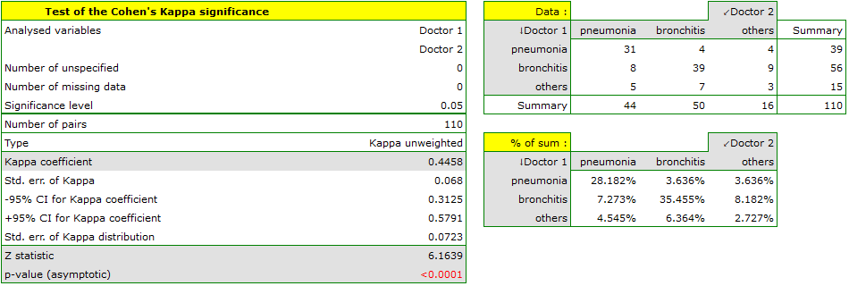
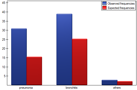
The agreement expressed by the coefficient \(\hat \kappa=44.58\%\) is lower than the agreement not adjusted for the chance of agreement.
Example 2. (radiology.pqs file)
Liver damage was assessed on radiological images using the following categories: no changes (1), mild changes (2), suspected cancer (3), cancer (4). The assessment was made by two independent radiologists based on a group of 70 patients. We want to check the agreement of the diagnosis made.
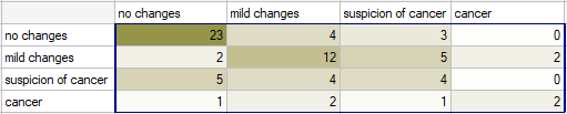
Because the diagnosis is made on an ordinal scale, the appropriate measure of agreement would be the weighted Kappa coefficient.
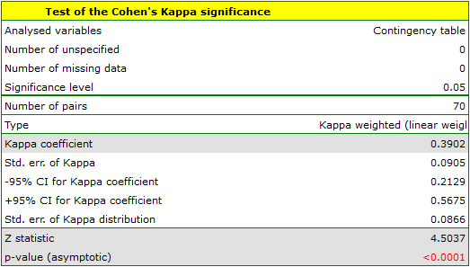
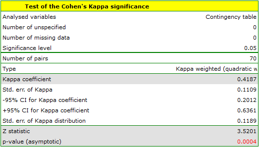
Because the data are concentrated mainly on the main diagonal of the matrix and in its immediate vicinity, the coefficient weighted by linear weights is lower than the coefficient determined using quadratic weights. If there were substantial disagreement concerning the two extreme cases, and the pair (no changes and cancer), located in the top-right corner of the table, occurred far more often, e.g. 15 times, then such a large lack of agreement would be more apparent when using quadratic weights (the Kappa coefficient would drop drastically) than when using linear weights.
Linear weights
Example weights for a 5x5 matrix:
| 1 | 0.75 | 0.5 | 0.25 | 0 |
| 0.75 | 1 | 0.75 | 0.5 | 0.25 |
| 0.5 | 0.75 | 1 | 0.75 | 0.5 |
| 0.25 | 0.5 | 0.75 | 1 | 0.75 |
| 0 | 0.25 | 0.5 | 0.75 | 1 |
Quadratic weights
Example weights for a 5x5 matrix:
| 1 | 0.9375 | 0.75 | 0.4375 | 0 |
| 0.9375 | 1 | 0.9375 | 0.75 | 0.4375 |
| 0.75 | 0.9375 | 1 | 0.9375 | 0.75 |
| 0.4375 | 0.75 | 0.9375 | 1 | 0.9375 |
| 0 | 0.4375 | 0.75 | 0.9375 | 1 |
Procedure:
To determine agreement using the Kappa coefficient, the data are presented as a table of observed frequencies \(O_{ij}\) (?), which is then transformed into a probability contingency table \(p_{ij}=O_{ij}/n\).
The Kappa coefficient (\(\hat \kappa\)) is then expressed by the formula:
where:
\(P_o=\sum_{i=1}^c\sum_{j=1}^c w_{ij}p_{ij}\),
\(P_e=\sum_{i=1}^c\sum_{j=1}^c w_{ij}p_{i.}p_{.i}\),
\(p_{i.}\), \(p_{.i}\) – the row and column totals of the probability contingency table.
The standard error for Kappa is expressed by the formula:
where:
\(\overline{w}_{i.}=\sum_{j=1}^{c}p_{.j}w_{ij}\),
\(\overline{w}_{.j}=\sum_{i=1}^{c}p_{i.}w_{ij}\).
The Z-test for the significance of the Cohen's Kappa coefficient (\(\hat \kappa\)) (Fleiss, 2003[63]) is used to verify the hypothesis about the agreement of the results of two measurements \(X^{(1)}\) and \(X^{(2)}\) of feature \(X\), and is based on the \(\hat \kappa\) coefficient calculated for the sample.
Hypotheses:
\(\begin{array}{cl} \mathcal{H}_0: & \kappa= 0, \\ \mathcal{H}_1: & \kappa \ne 0. \end{array}\)
Formulas:
The test statistic is defined by:
where:
The \(Z\) statistic asymptotically (for large sample sizes) has the normal distribution.
The \(p\) value, determined on the basis of the test statistic, is compared with the significance level \(\alpha\): if \(p \le \alpha\), we reject \(\mathcal{H}_0\) in favor of \(\mathcal{H}_1\); if \(p > \alpha\), there is no reason to reject \(\mathcal{H}_0\).