 PQStat
The Q-Cochran ANOVA
When to use this test:
The Q-Cochran analysis of variance (Cochran, 1950[41]) extends the McNemar test to \(k\geq2\) dependent groups. It lets you check whether the results of several measurements of a two-valued feature (e.g. correct/wrong answer) are symmetric, i.e. whether the proportion of one of the values is the same across all measurements.
Assumptions
- measurement on a nominal scale (dichotomous variables, i.e. with 2 categories, coded as 0 and 1),
- a dependent model.
How to set up the analysis
Statistics \(\to\) Nonparametric tests (unordered categories) \(\to\) Q-Cochran ANOVA (or via the Wizard).
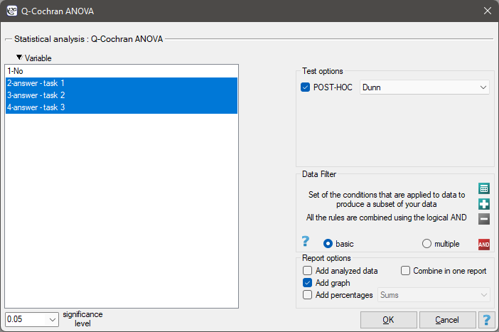
Performing and interpreting the analysis
Example 1. (test.pqs file)
We want to compare the difficulty of 3 test questions. To do this, we select a sample of 20 people from the population the test is aimed at. Each person in the sample answers 3 questions from the test, after which we check the correctness of the answers (an answer can be correct or wrong). The results are shown in the table below.
| No. | Question 1 answer | Question 2 answer | Question 3 answer |
| 1 | correct | correct | wrong |
| 2 | wrong | correct | wrong |
| 3 | correct | correct | correct |
| 4 | wrong | correct | wrong |
| 5 | wrong | correct | wrong |
| 6 | wrong | correct | correct |
| 7 | wrong | wrong | wrong |
| 8 | wrong | correct | wrong |
| 9 | correct | correct | wrong |
| 10 | wrong | correct | wrong |
| 11 | wrong | wrong | wrong |
| 12 | wrong | wrong | correct |
| 13 | wrong | correct | wrong |
| 14 | wrong | wrong | correct |
| 15 | correct | wrong | wrong |
| 16 | wrong | wrong | wrong |
| 17 | wrong | correct | wrong |
| 18 | wrong | correct | wrong |
| 19 | wrong | wrong | wrong |
| 20 | correct | correct | wrong |
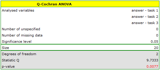
We resume the analysis with the  button to perform a POST-HOC test, and in the test options window we select the POST-HOC Dunn.
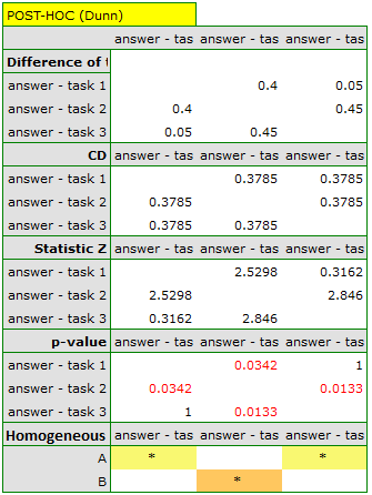
The POST-HOC analysis performed shows that the differences concern question 2 and 1, and question 2 and 3. The difference is that question 2 is easier than questions 1 and 3 (the number of correct answers is higher there).
Hypotheses:
\(\begin{array}{cl} \mathcal{H}_0: & ''incompatible'' observed frequencies are all equal, \\ \mathcal{H}_1: & ''incompatible'' observed frequencies are not all equal, \end{array}\)
where ”incompatible” observed frequencies are the observed frequencies calculated when the value of the analysed feature differs across successive measurements.
Formulas:
The test statistic is defined by:
where:
\(T=\sum_{i=1}^n\sum_{j=1}^kx_{ij}\),
\(R=\sum_{i=1}^n\left(\sum_{j=1}^kx_{ij}\right)^2\),
\(C=\sum_{j=1}^k\left(\sum_{i=1}^nx_{ij}\right)^2\),
\(x_{ij}\) – the value of the \(j\)-th measurement for the \(i\)-th object (i.e. 0 or 1).
This statistic asymptotically (for large sample sizes) has the \(\chi^2\) distribution with \(df=k-1\) degrees of freedom.
The \(p\) value, determined on the basis of the test statistic, is compared with the significance level \(\alpha\): if \(p \le \alpha\), we reject \(\mathcal{H}_0\) in favor of \(\mathcal{H}_1\); if \(p > \alpha\), there is no reason to reject \(\mathcal{H}_0\).
POST-HOC tests
An introduction to contrasts and POST-HOC tests is provided in section Contrasts and POST-HOC tests, which concerns the one-way analysis of variance.
The Dunn test
Used for simple comparisons (the counts in each measurement are always the same).
Example – simple comparisons (for the difference in proportion for one selected pair of measurements).
Hypotheses:
- \(\mathfrak{(i)}\)
The critical difference is calculated using the formula:
\[ CD=Z_{\frac{\alpha}{c}}\sqrt{2\frac{kT-R}{n^2k(k-1)}}, \]where \(Z_{\frac{\alpha}{c}}\) is the critical value (statistic) of the normal distribution for the significance level \(\alpha\) adjusted for the number of possible simple comparisons \(c\).
- \(\mathfrak{(ii)}\)
The test statistic is defined by:
\[ Z=\frac{\sum_{j=1}^k c_jp_j}{\sqrt{2\frac{kT-R}{n^2k(k-1)}}}, \]where \(p_j\) – proportion of the \(j\)-th measurement \((j=1,2,...k)\). This statistic asymptotically (for large sample sizes) has the normal distribution, and the \(p\) value is adjusted for the number of possible simple comparisons \(c\).