The Chi-square test for multidimensional contingency tables

When to use this test:

The \(\chi^2\) test for multidimensional contingency tables is used when we want to check the dependence between more than two features at once – it is an extension of the \(\chi^2\) test for (\(R\times C\)) tables to three or more features.

Assumptions

measurement on a nominal scale – any ordering of categories is not taken into account,
an independent model,
large expected frequencies according to the Cochran interpretation (1952)[42].

How to set up the analysis

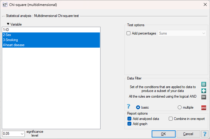
Statistics \(\to\) NonParametric tests (unordered categories) \(\to\) Chi-square (multidimensional) (or via the Wizard).

Step 1. Indicate all the analysed features (three or more).

Step 2. Run the analysis.

Note! This test can only be calculated on the basis of raw data.

Performance and interpretation

Example 1. (heart_disease.pqs file)
A sample of 200 people was examined for three features: sex (\(X_1\): f, m), cigarette smoking (\(X_2\): yes, no), and the presence of heart disease (\(X_3\): yes, no). The aim of the study was to check whether there is a dependence between these three features in the analysed population.

\(\chi^2=52.382342\), \(df=4\), \(p<0.000001\) (statistically significant, \(\alpha=0.05\))

There is a statistically significant dependence between sex, cigarette smoking, and the presence of heart disease in the analysed population.

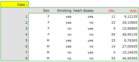
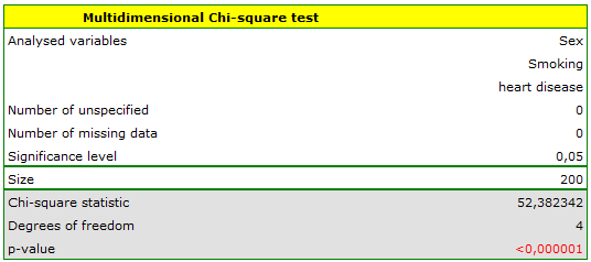
The expected frequencies shown in the data window are large enough (Cochran's condition is satisfied), so the test result is reliable. Comparing the observed and expected frequencies shows where the dependence is strongest: among male smokers, heart disease occurs much more often than would be expected under no dependence (25 observed cases versus 8.76 expected) – almost three times more often than expected. The opposite pattern is seen among male non-smokers: heart disease occurs much less often than expected (4 observed cases versus 15.25 expected). Among women, the deviations between observed and expected frequencies are clearly smaller. The dependence therefore mainly concerns men – for them, cigarette smoking is associated with a markedly increased risk of heart disease.

FOR THOSE INTERESTED

Hypotheses:

\[ \begin{array}{cl} \mathcal{H}_0: & O_{ij...}=E_{ij...} \text{ for all categories,}\\ \mathcal{H}_1: & O_{ij...} \neq E_{ij...} \text{ for at least one category,} \end{array} \]

where \(O_{ij...}\) and \(E_{ij...}\) are observed frequencies in a contingency table and the corresponding expected frequencies.

Formulas:

The test statistic is defined by:

\[ \chi^2=\sum_{i=1}^r\sum_{j=1}^c\sum...\sum\frac{(O_{ij...}-E_{ij...})^2}{E_{ij...}}. \]

This statistic asymptotically (for large expected frequencies) has the \(\chi^2\) distribution with a number of degrees of freedom calculated, for a 3-dimensional table, using the formula:

\[ df = (r - l)(c - 1)(l - 1) + (r- l)(c- 1) + (r- 1)(l- 1) + (c- 1)(l- 1). \]