The Chi-square test for small tables

When to use this test:

The \(\chi^2\) test for \(2\times 2\) tables (also known as Pearson's Chi-square test, Karl Pearson 1900) is used when we want to check whether two features with two categories each (e.g. sex and exam passing) are related. It is a special case of the \(\chi^2\) test for \(r\times c\) tables for the smallest possible table.

Assumptions

measurement on a nominal scale,
an independent model,
a \(2\times 2\) contingency table (see table (1)).

How to set up the analysis

Statistics \(\to\) NonParametric tests \(\to\) Chi-square, Fisher, OR/RR (or via the Wizard).

Step 1. Indicate the two features whose dependence you want to check.

Step 2. Run the analysis.

Note! When the expected frequencies in the table are small (below 5), it is better to base the conclusion on the test with Yates correction, Fisher's exact test, or the mid-p test, rather than the basic \(\chi^2\) test – all are calculated automatically together with the basic test.

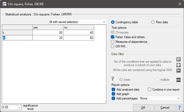
Performance and interpretation

Example 1. (sex-exam.pqs file)
There is a sample of 170 people (\(n=170\)), for whom 2 features are analysed (\(X\)=sex, \(Y\)=exam passing). Each of these features occurs in two categories (\(X_1\)=f, \(X_2\)=m, \(Y_1\)=yes, \(Y_2\)=no). Based on this sample, we would like to find out whether there is a dependence between sex and exam passing in the analysed population. The data distribution is shown in the contingency table below:

Observed frequencies		exam passing
\(O_{ij}\)		yes	no	total
sex	f	50	40	90
	m	20	60	80
	total	70	100	170

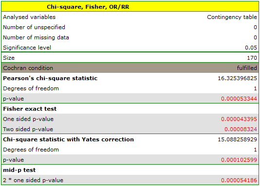
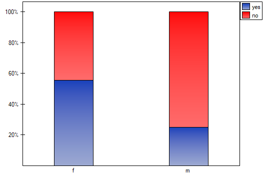
\(p=0.000053\) (chi-square test, statistically significant, \(\alpha=0.05\))

There is a dependence between sex and exam passing in the analysed population.

The table of expected frequencies contains no values below 5, so Cochran's condition is satisfied – the basic \(\chi^2\) test could be applied directly. The other test variants lead to the same conclusion: the test with Yates correction (\(p=0.000103\)), Fisher's exact test (\(p=0.000083\)), and the mid-p test (\(p=0.000054\)).

FOR THOSE INTERESTED

Hypotheses:

\[ \begin{array}{cl} \mathcal{H}_0: & \text{there is no dependence between the analysed features in the population,}\\ \mathcal{H}_1: & \text{there is a dependence between the analysed features in the population.} \end{array} \]

Formulas: The test statistic is defined by:

\[ \chi^2=\sum_{i=1}^2\sum_{j=1}^2\frac{(O_{ij}-E_{ij})^2}{E_{ij}}. \]

This statistic asymptotically (for large expected frequencies) has the \(\chi^2\) distribution with 1 degree of freedom.