MULTIPLE COMPARISONS

When to use:

Simultaneously testing many hypotheses (the so-called family of hypotheses) carries the risk of an increase in the error \(\alpha\), which is the main problem in the field of multiple comparisons. When the error \(\alpha\) increases, it means that we reject the null hypothesis too often when it is in fact true – that is, we too often indicate that differences exist when in reality they do not. To guard against an increase in \(\alpha\), one strategy is to adjust (reduce) the level of \(\alpha\), or to adjust (increase) the \(p\) values of the tests accordingly.

Note! A family of hypotheses can be defined in many ways. Most often these are hypotheses arising within a POST-HOC procedure, i.e. performing many tests as part of a simultaneous comparison of several groups studied. Such a family can also be formed by tests performed as part of a Hotelling-type analysis. Families of hypotheses also occur in many geographical analyses. Wherever many smaller hypotheses are analysed within an overall hypothesis, a multiple-comparisons correction may apply.

How to set up the analysis

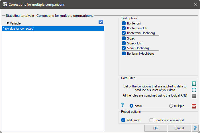
To perform a multiple-comparisons correction, enter successive \(p\) values into a single column of the data sheet. The settings window for the multiple comparisons options is opened via the Statistics\(\to\)Correction for multiple comparisons menu.

Performing and interpreting the analysis

Continuation of Example 1 (jobSatisfaction.pqs file): this study examined whether the level of job satisfaction was the same across four education categories. Here, the family of hypotheses consisted of the hypotheses resulting from comparing all groups pairwise. To compare all 4 groups, 6 pairs of comparisons were formed – in each case the null hypothesis stated that there was no difference in satisfaction for the pair analysed. To make use of several of the proposed multiple-comparisons corrections, the analysis was performed using the uncorrected Dunn POST-HOC test.

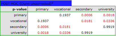
The \(p\) values obtained in this way were entered as the data for the multiple-comparisons correction, yielding the following results:

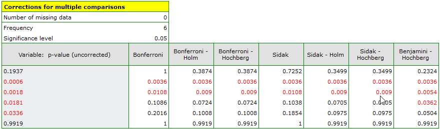
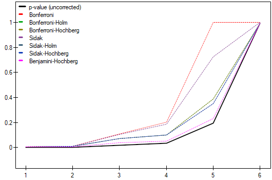
statistically significant differences for 2 (or 3, with the Benjamini-Hochberg correction) of the 6 pairs of comparisons, \(\alpha=0.05\)

The differences concern job satisfaction for primary versus secondary education, and primary versus higher education.

Only when the Benjamini-Hochberg correction is applied can differences be located in three pairs of comparisons.

Other examples of applying the multiple-comparisons correction: Example 1 and Example 2 (Hotelling-type analysis).

FOR THOSE INTERESTED

If we denote the number of hypotheses tested by \(c\), the corrections for multiple comparisons can be described as follows:

The Bonferroni correction
The best known and, at the same time, the most conservative of the corrections[2]. It consists in multiplying each test probability by the total number of tests performed (or dividing the significance level by that number).
Formula – \(p\)-value adjustment:

\[ p_{(Bonferroni,i)}=p_i\cdot c \]

Formula – significance-level \(\alpha\) adjustment:

\[ \alpha_{(Bonferroni, i)}=\frac{\alpha_i}{c} \]

The Sidak correction
The Sidak correction (1967)[155] has greater power than the Bonferroni correction, which is why it is increasingly used.
Formula – \(p\)-value adjustment:

\[ p_{(Sidak, i)}=1-(1-p_i)^{c} \]

Formula – significance-level \(\alpha\) adjustment:

\[ \alpha_{(Sidak, i)}=1-(1-\alpha_i)^{1/c} \]

The Bonferroni-Holm correction
Consists in applying Holm's (1979)[84] multi-step procedure to the Bonferroni correction. The procedure begins by sorting the successive \(p_i\) values \((p_1, p_2,...p_c)\) in ascending order. The Bonferroni correction is then applied to each successive \(p_i\) value (with a corresponding reduction in the number of hypotheses remaining to be tested). As a result, all hypotheses tested after the first statistically non-significant \(p_i\) value are also non-significant.
Formula – \(p\)-value adjustment:

\[ p_{(Bonferroni, i)}=p_i\cdot (c-i+1) \]

The Sidak-Holm correction
Consists in applying Holm's multi-step procedure to the Sidak correction, analogously to the Bonferroni-Holm correction above.
Formula – \(p\)-value adjustment:

\[ p_{(Sidak, i)}=1-(1-p_i)^{c-i+1} \]

The Bonferroni-Hochberg correction
Consists in applying Hochberg's (1988)[36] multi-step procedure to the Bonferroni correction. The procedure begins by sorting the successive \(p_i\) values \((p_c,p_{c-1},...,p_1)\) in descending order. The Bonferroni correction is then applied to each successive \(p_i\) value (with a corresponding reduction in the number of hypotheses remaining to be tested). As a result, all hypotheses tested after the first statistically non-significant \(p_i\) value are also non-significant.
Formula – \(p\)-value adjustment:

\[ p_{(Bonferroni, i)}=p_i\cdot (c-i+1) \]

The Sidak-Hochberg correction
Consists in applying Hochberg's multi-step procedure to the Sidak correction, analogously to the Bonferroni-Hochberg correction above.
Formula – \(p\)-value adjustment:

\[ p_{(Sidak, i)}=1-(1-p_i)^{c-i+1} \]

The Benjamini-Hochberg correction
Consists in applying Hochberg's multi-step procedure to Benjamini's (1995)[19] correction, which is a modified version of the Bonferroni correction. The procedure begins by sorting the successive \(p_i\) values \((p_c,p_{c-1},...,p_1)\) in descending order. Benjamini's correction is then applied to each successive \(p_i\) value (with a corresponding reduction in the number of hypotheses remaining to be tested). As a result, all hypotheses tested after the first statistically non-significant \(p_i\) value are also non-significant. Of the corrections proposed, it has the greatest power – it does not directly control the error \(\alpha\), but minimises the expected proportion of false differences among the differences detected.
Formula – \(p\)-value adjustment:

\[ p_{(BH, i)}=p_i\frac{c}{i} \]