 PQStat

One-dimensional normality tests
When to use:
A variety of tests may be applicable when examining the normality of a distribution, each of which pays attention to slightly different aspects of the Gaussian distribution. It is impossible to identify a single test that is good for every possible data set. Testing for normality of distribution can be done for variables or for differences determined from two variables.
Assumptions
- measurement on an interval scale.
Definitions of measures
The Kolmogorov-Smirnov test – proposed by Kolmogorov (1933)[97], it is a relatively conservative test (it is harder to prove non-normality of the distribution using it). It is based on determining the distance between the empirical and theoretical cumulative distribution functions of the normal distribution. It is recommended for large samples, but should be used when the mean (\(\mu\)) and standard deviation (\(\sigma\)) of the population from which the sample is drawn are known – one can then check whether the distribution matches the distribution defined by the given mean and standard deviation.
The Lilliefors test – a test proposed by Lilliefors (1967, 1969, 1973)[106][107][108]. It is a correction of the Kolmogorov-Smirnov test, used when the mean and standard deviation of the population from which the sample is drawn are not known. It is considered slightly less conservative than the Kolmogorov-Smirnov test.
The Shapiro-Wilk test – proposed by Shapiro and Wilk (1965)[152] for small samples, and later adapted for larger samples (up to 5000 objects) by Royston (1992)[145][146]. This test has relatively high power, which makes it easier to demonstrate non-normality of the distribution. The idea behind the test is illustrated by the Q-Q plot.
The D'Agostino-Pearson test – different types of statistical analysis that assume normality are sensitive to different degrees to different kinds of departure from this assumption. Tests referring to means in their hypotheses are assumed to be more sensitive to skewness, while tests comparing variances depend more heavily on kurtosis. A normal distribution should be characterised by zero skewness and zero kurtosis \(g_2\) (or \(b_2\) close to the value three). When the distribution is found not to be normal by the D'Agostino test (1973)[3], one can check whether this is caused by high skewness or kurtosis via the skewness test and the kurtosis test. Like the Shapiro-Wilk test, the D'Agostino test has greater power than the Kolmogorov-Smirnov and Lilliefors tests (D'Agostino, 1990[4]).
The Quantile-Quantile plot (Q-Q plot) – used to show the correspondence between two distributions. When checking agreement with a normal distribution, it checks the agreement of the data distribution (empirical distribution) with the theoretical Gaussian distribution. From it, one can visually check how well the normal-distribution curve fits the data. If the quantiles of the theoretical and empirical distributions match, the points fall along the line \(y=x\). The horizontal axis represents the quantiles of the normal distribution, and the vertical axis the quantiles of the data distribution.
Very different deviations from the normal distribution are possible – the interpretation of a few of the most common ones is described below:
- the data lie along the line, but a few points deviate strongly from it – there are outliers in the data;
- points on the left side of the plot lie above the line, and on the right side below it – the distribution has a greater presence of values far from the mean than a normal distribution (negative kurtosis);
- points on the left side of the plot lie below the line, and on the right side above it – the distribution has a smaller presence of values far from the mean than a normal distribution (positive kurtosis);
- points on both the left and right sides of the plot lie above the line – the distribution is right-skewed (positive skewness);
- points on both the left and right sides of the plot lie below the line – the distribution is left-skewed (negative skewness).
How to set up the analysis
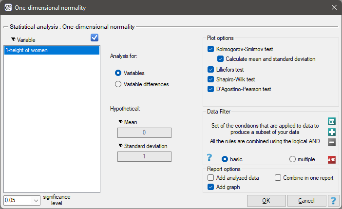
Statistics \(\to\) Normality tests \(\to\) One-dimensional normality (or via the Wizard).
Performing and interpreting the analysis
Example 1. (Gauss.pqs file)
Women's height
Let us assume that women's height is a feature for which the average value is 168 cm. Most of the women we meet every day are of a height not significantly different from this average. Of course there are women who are quite short, and also very tall, but relatively rarely. Since very low and very high values occur rarely, and average values occur often, we can expect that the distribution of height is normal. To find out, 300 randomly selected women were measured.
Since we do not know the mean or standard deviation for women's height, but only have assumptions about these quantities, they will be determined from the sample.
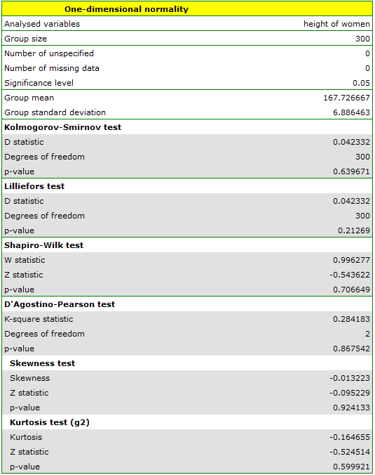
The test examining skewness and kurtosis also shows no deviations. In the column chart, we presented the height distribution as 10 columns. The largest group consists of women with a height between 167 cm and 171 cm, while the smallest groups are women shorter than 150 cm or taller than 184 cm. The bell curve of the normal distribution seems to describe this distribution well.
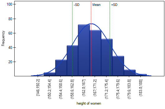
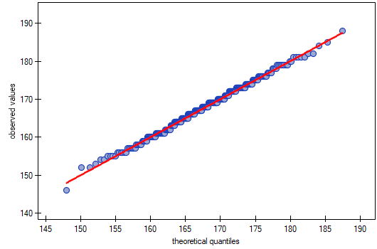
On the quantile-quantile plot, the points lie almost perfectly on the line, which also indicates a very good fit to the normal distribution.
The normal distribution can therefore be regarded as the distribution characterising women's height in the population studied.
Example 2. (Gauss.pqs file)
Income
Suppose we study people's income in a certain country. We expect that most people's income will be average; however, there will be no people earning very little (below the minimum wage set by the authorities), while there will be people earning very much (company presidents), of whom there are relatively few. To check whether people's income in the country studied has a normal distribution, information on the income of 264 randomly selected people was collected.
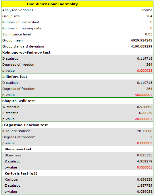
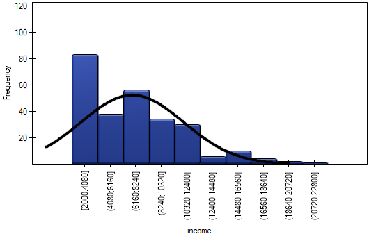
The positive and statistically significant (\(p<\alpha\)) skewness value indicates that the right tail of the function is too long. The distribution is also more slender than the normal distribution, but this difference is not statistically significant (kurtosis test).
On the quantile-quantile plot, the deviation from the normal distribution is shown by right-hand skewness, i.e. the position of the initial and final points of the plot well above the line.
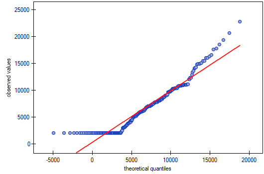
As a result, the data collected do not support agreement between the income distribution and a normal distribution.
Hypotheses for normality-of-distribution tests:
Interpretation: the \(p\) value, determined on the basis of the test statistic of the chosen test, is compared with the significance level \(\alpha\): if \(p \le \alpha\), we reject \(\mathcal{H}_0\) in favor of \(\mathcal{H}_1\); if \(p > \alpha\), there is no reason to reject \(\mathcal{H}_0\).
The Kolmogorov-Smirnov test
Formula: on the basis of the sample data collected in a cumulative frequency distribution, and the corresponding values of the area under the theoretical normal-distribution curve, we determine the value of the test statistic \(D\):
where:
\(F_n(x)\) – the empirical cumulative distribution function calculated at successive points of the distribution, for an \(n\)-element sample,
\(F(x)\) – the theoretical cumulative distribution function of the normal distribution.
The test statistic has the Kolmogorov-Smirnov distribution.
The Lilliefors test
Explanation: the test statistic \(D\) is calculated using the same formula as the Kolmogorov-Smirnov test, but has the Lilliefors distribution.
The Shapiro-Wilk test
Formulas: the Shapiro-Wilk test statistic is defined by:
where:
\(a_i\) – coefficients determined on the basis of the expected values of the ordered statistics, assigned weights, and the covariance matrix,
\(\overline{x}\) – the mean of the sample data.
This statistic is transformed into a statistic with a normal distribution:
where \(g(W)\), \(\mu\), and \(\sigma\) depend on the sample size:
for small sample sizes \(n\in\langle4;12)\):
\(g(W)=-\ln(\gamma-\ln(1-W))\),
\(\gamma=0.459n-2.273\),
\(\mu=-0.0006714n^3+0.025054n^2-0.39978n+0.5440\),
\(\sigma=\exp(-0.0020322n^3+0.062767n^2-0.77857n+1.3822)\);for large sample sizes \(n\in\langle12;5000\rangle\):
\(g(W)=\ln(1-W)\),
\(\mu=0.0038915u^3-0.083751u^2-0.31082u-1.5851\),
\(\sigma=\exp(0.0030302u^2-0.082676u-0.4803)\),
\(u=\ln(n)\).
The D'Agostino-Pearson test
Formulas: the test statistic is defined by:
where:
\(Z_A^2\) – the test statistic of the skewness test,
\(Z_K^2\) – the test statistic of the kurtosis test.
This statistic asymptotically has the \(\chi^2\) distribution with two degrees of freedom.
The D'Agostino skewness test
Hypotheses:
Formulas: the test statistic is defined by:
where:
\(Y=\sqrt{(b_1)}\sqrt{\frac{(n+1)(n+3)}{6(n-2)}}\),
\(\sqrt{(b_1)}=\frac{m_3}{m_2^{(3/2)}}\),
\(m_k=\frac{\sum_{i=1}^{n}(x_i-\overline{x})^k}{n}\),
\(\beta(\sqrt{(b_1)})=\frac{3(n^2+27n-70)(n+1)(n+3)}{(n-2)(n+5)(n+7)(n+9)}\),
\(W^2=-1+\sqrt{2(\beta(\sqrt{(b_1)})-1}\),
\(\delta=\frac{1}{\sqrt{\ln W}}\),
\(\alpha=\sqrt{\frac{2}{W^2-1}}\).
The statistic \(Z\) asymptotically (for large sample sizes) has the normal distribution.
The D'Agostino kurtosis test
Hypotheses:
Formulas: the test statistic is defined by:
where:
\(E(b_2)=\frac{3(n-1)}{n+1}\),
\(b_2=\frac{m_4}{m_2^2}\),
\(var(b_2)=\frac{24n(n-2)(n-3)}{(n+1)^2(n+3)(n+5)}\),
\(x=\frac{b_2-E(b_2)}{\sqrt{var(b_2)}}\),
\(\sqrt{\beta(b_2)}=\frac{6(n^2-5n+2)}{(n+7)(n+9)}\sqrt{\frac{6(n+3)(n+5)}{n(n-2)(n-5)}}\),
\(H=6+\frac{8}{\sqrt{\beta(b_2)}}\left(\frac{2}{\sqrt{\beta(b_2)}}+\sqrt{1+\frac{4}{\beta(b_2)}}\right)\).
The statistic \(Z\) asymptotically (for large sample sizes) has the normal distribution.