Factorial ANOVA – GLM

When to use:

Factorial analysis of variance GLM is an extension of one-way analysis of variance (ANOVA) for independent groups and multiple linear regression. The acronym GLM (general linear model) stands for General Linear Model. GLM analysis typically involves the use of linear regression models to calculate various composite ANOVA comparisons.

Factorial ANOVA is a type of analysis of variance in which we can use either one or many factors to separate the groups being compared. Variables that are interactions of the indicated factors may also take part in the analysis. When ANOVA includes more than one factor, these factors are confounded with each other. Factorial ANOVA requires that the factors be divided into individual categories (i.e. independent populations), e.g. factor \(A\): sex, divided into male and female; factor \(B\): education, divided into primary, vocational, secondary, and higher education. The interaction of factor \(A*B\) is also divided into categories – in this case, we obtain eight categories.

Example of equivalent analyses that can be performed through GLM. The analyses in each row of the table are equivalent in the sense that their results are the same, although they need not be identical. The study concerns the income of a certain group of people, about whom we have some additional information, such as sex and education.

income and...	ANOVA	Multiple regression
	t-test for independent groups	dependence of income (\(Y\)) on sex (\(X\))
sex	\(\star\) comparing income for women with income for men	\(\star\) sex as a column with two categories
	One-way ANOVA	dependence of income (\(Y\)) on education (\(X\))
education	\(\star\) comparing income for people with different education	\(\star\) education broken down into dummy variables
	(primary, vocational, secondary, higher)
	Multi-factor ANOVA	dependence of income (\(Y\)) on sex (\(X_1\))
sex,	\(\star\) comparing income for women with income for men	and education (\(X_2\))
	taking education into account as a confounding variable	\(\star\) sex as a column with two categories
education	\(\star\) comparing income for people with different education	\(\star\) education broken down into dummy variables
	(primary, vocational, secondary, higher)
	taking sex into account as a confounding variable	both variables are mutually confounding
	Multi-factor ANOVA	dependence of income (\(Y\)) on sex (\(X_1\)),
sex,	\(\star\) comparing income for women with income for men	on education (\(X_2\)), and on the
	taking other variables in the model into account	*interaction of sex and education (\(X_1X_2\))**
education,	\(\star\) comparing income for people with different education	\(\star\) sex as a column with two categories
	(primary, vocational, secondary, higher)	\(\star\) education broken down into dummy variables
	taking other variables in the model into account	\(\star\) interaction is the product of sex and education
sex*education	\(\star\) comparing income for people with different
	education and sex (in interaction)	the variables in the model are mutually confounding
	taking other variables in the model into account

GLM analysis can be used in any of the above cases, but since multiple regression analysis, like one-way ANOVA, has been discussed in a separate chapter, in this chapter we will present the use of GLM in multi-factor ANOVA.

Assumptions

measurement on an interval scale,
the samples come from a population with a normal distribution (normality of the variables or model residuals),
an independent model,
equality of variances of the variables studied in the populations compared.

Definitions of measures

The influence of confounding factors – although all factors participating in the analysis are confounded with each other, their influence on the significance of individual factors can be controlled. There are three ways in which, when examining the significance of individual factors, the influence of confounding variables can be taken into account. They depend on how the sum of squares is calculated:

Type I sums of squares – depend on the order in which the individual factors appear in the model. This type of sum of squares means that the significance of the factor being interpreted is adjusted for those variables whose order in the model was earlier, while the remaining variables in the model only indirectly affect the result of the analysis.
Use: recommended when the study is fully balanced, with equal or proportional counts in each category, including when interactions are present. Not recommended when the study is unbalanced (different counts in each category) and/or interactions are present.

Type II sums of squares – the significance of the factor being interpreted is adjusted for those variables whose order is the same or lower, while the remaining variables in the model only indirectly affect the result of the analysis.
Use: recommended when the study is fully balanced, with equal or proportional counts in each category, including when interactions are present. Not recommended when the study is unbalanced (different counts in each category) and/or interactions are present.

Type III sums of squares – the significance of the factor being interpreted is adjusted for all other variables in the model. We recommend using this type of sum of squares when effect coding is selected.
Use: recommended when the study is balanced or unbalanced, including when interactions are present. Not recommended when the study contains subclasses with missing observations.

Note! In PQStat, Type III sums of squares are selected by default because of their universality. The effect coding option, described in the Preparation of variables for analysis in multivariate models section, is also selected by default. Note that the choice of appropriate coding affects both the interpretation of the model coefficients and the significance of individual factors in factorial ANOVA – especially with unbalanced designs.

ANOVA approach vs. regression approach – ANOVA-type analysis and regression models are treated equivalently, and in the general case their hypotheses converge. When interpreting these hypotheses, it should be remembered that the hypotheses for a given factor are adjusted for those other factors that a given analysis includes. The model approach assumes the following regression model:

\[ Y=\mu+\alpha_iA_i+\beta_jB_j+(\alpha\beta)_kB_k+\epsilon, \]

where:
\(Y\) – the dependent variable, explained by the model,
\(\mu\) – the overall mean of variable \(Y\) (if effect coding was used),
\(A_i, B_j, AB_k\) – factors – independent, explanatory variables,
\(\alpha_i,\beta_i,\alpha\beta_i\) – parameters,
\(\epsilon\) – the random component (model residual).

Coding – the analysis results obtained (in particular the constructed regression model) and the interpretation of the hypotheses also depend on the coding method. PQStat offers dummy coding and effect coding. By default, the program selects effect coding – unchecking this option is equivalent to selecting dummy coding.

Note! When using Type III sums of squares, when interactions are present, it is advisable to use effect coding.

How to set up the analysis

Statistics \(\to\) Multivariate models \(\to\) Factorial ANOVA GLM.

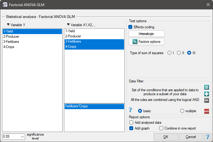
Performing and interpreting the analysis

Example 1. (yield.pqs file)
To increase crop yields, fertilizers are being developed using increasingly newer technologies. On the basis of an experiment, the researchers want to find out which of three blends of new fertilizers is the most effective. The crops were grown on two different farms and involved sowing wheat, rye, oats, and barley. Yield was reported as a % (compared to the yield obtained without fertilization).

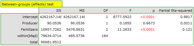
First, we want to check whether: (1) the average yields obtained when fertilizing with blend X are the same as those obtained with blend Y and the same as those obtained with blend Z (regardless of the farm growing the crop); (2) the average yields obtained on farm 1 are the same as on farm 2 (regardless of the fertilizer blend used). Equivalently, using a regression approach: (1) the coefficients indicating the change in yield obtained when the fertilizer applied changes are zero (regardless of the farm growing the crop); (2) the coefficient indicating the change in yield obtained when the farm growing the crop changes is zero. In a second application of GLM, we will check whether: (3) the average yields obtained from growing individual cereals are the same when different fertilizer treatments are used.

Hypotheses 1) and 2) – ANOVA approach
We will conduct the analysis using the third type of sum of squares and effect coding.

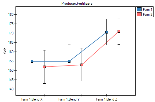
fertilizer blend: \(p=0.000026\), partial Eta-squared \(\approx\) 12%; farm: \(p=0.667289\), partial Eta-squared = 0.1%

Yield depends significantly on the fertilizer blend applied, but does not depend on the farm on which the crop was grown.

After selecting the observed or expected averages in the Factor Options window, we can represent these differences graphically on plots showing the average yields for each fertilizer blend applied. The exact values of the averages can be read from the descriptive statistics table.

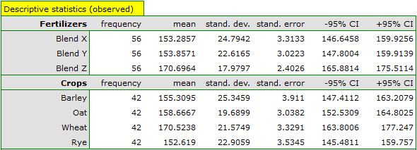
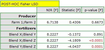
We can check where the differences are located using post-hoc tests. Fisher's LSD post-hoc test indicates that the most favourable results are obtained using blend Z – the yield obtained is on average 170.7% of the yield that would be obtained without fertilization. The remaining blends do not differ statistically significantly in the yield obtained. Since the model analysed the farm on which the crops were grown simultaneously, we can say that the advantage of blend Z is independent of the farm on which the sowing was done.

Regression approach
An analogous interpretation can be obtained using the regression model, although the interpretation here is somewhat more difficult – the difficulty arises from the need to determine the coding method and the choice of reference category. Let us first look at the results obtained with dummy coding, which we can obtain by unchecking the effect coding option. The analysis automatically took the alphabetically first level as the reference level – for fertilizers, this level was blend X; for farms, it was farm 1.

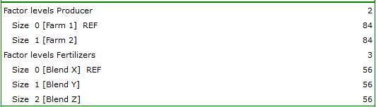
The analysis of the model coefficients resembles the analysis of post-hoc tests, with the difference that we compare only to the reference category. So if we compare all fertilizer blends to blend X, we can see that only using blend Z produced significantly higher results (p=0.000047) – these results are higher by 17.410714 (recall that the means were, respectively, 153.285714 for blend X and 170.696429 for blend Z). Comparing farms is simple, since we only have two farms to compare, and the result obtained is the result of comparing farm 2 with farm 1, which was the reference category. This time the difference obtained was small (-1.464286) and not statistically significant (0.667289).

Using effect coding, we also choose a reference category, but the magnitude of the coefficients and their significance is related not to the chosen reference category but to the overall average yield obtained, recorded in the model as the intercept (159.279762).

Compared to the overall average, we find quite a few differences: the yield obtained when fertilizing with blend Y is 5.422619 lower than the overall average, and with blend Z, 11.416667 higher. Both differences are statistically significant.

An undeniable advantage of building a regression model is the possibility of using its formula to predict the yields obtained. The models built are as follows:
For dummy coding: \(yield=154.017857+0.571429\cdot blendY + 17.410714\cdot blendZ-1.464286\cdot farm2\)
For effect coding: \(yield=159.279762-5.422619\cdot blendY + 11.416667 \cdot blendZ-0.732143 \cdot farm2\)

To be able to use the selected model for forecasting, go to the multiple regression – prediction menu and make a prediction based on the new data. The preparation of the data depends on how it is coded.

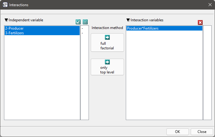
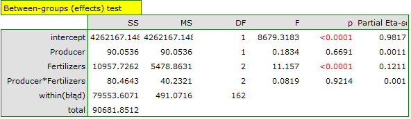
Based on all the results obtained, we do not suspect that yield depends on the interaction between the types of fertilizer used and the farm growing the crop. Most often, the presence of an interaction can be seen on the plot as clearly intersecting lines. Here, the two lines were almost parallel and close enough to each other that the difference between farms was not statistically significant. Although intersecting lines usually indicate the presence of an interaction, it should be remembered that when the lines are close to each other, their accidental crossing is very likely, meaning the interaction will not be statistically significant. However, to be sure, we will check whether there is an interaction in our case. To do this, we will select both variables once again in the interaction window and move them to the list of interactions on the right side of the window, then repeat the analysis.

interaction blend*farm: \(p=0.921377\) (not statistically significant)

We confirmed our suspicion that there is no significant interaction – in this case, a simpler model, i.e. without interaction, is recommended.

Hypothesis 3)
We encounter a different situation when examining the yield obtained depending on the fertilizer dose applied and the type of cereal grown.

We will perform an analysis that, besides the main effects, also takes interactions into account.

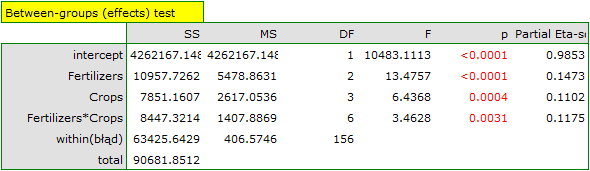
interaction fertilizer*cereal type: \(p=0.003066\) (statistically significant)

We should use the model with interactions, and the description of the results obtained should focus on this interaction.

In the ANOVA approach, the hypothesis concerning the interaction concerns all possible pairs of means, i.e. the average yields obtained when fertilizing each type of cereal with each fertilizer blend are equal. In the regression approach, we would say that the coefficients determining the change in yield obtained when the fertilizer applied and the type of crop change are zero.

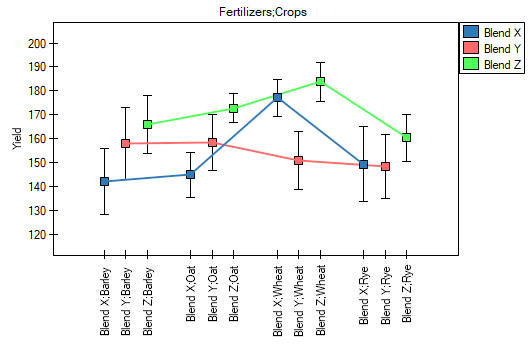
Based on the plot (and the averages recorded in the table), we can see that by far the best yields are obtained with blend Z, regardless of the type of cereal grown.

On the other hand, blend X and blend Y produce worse yields than blend Z, and there is also an interaction effect between them. This is manifested by the fact that wheat crops yield an unusually high yield when blend X is applied, compared to the wheat yield obtained when blend Y is applied, while barley and oat crops yield better when blend Y is applied. We can check the differences obtained in more detail by performing post-hoc tests. An excerpt from this report is given below:

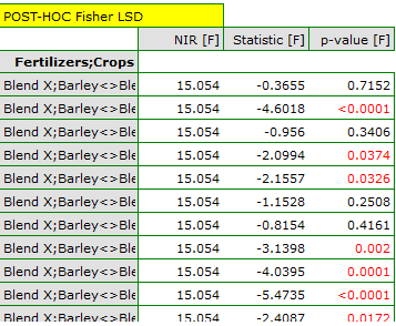
The result of Fisher's post-hoc test is extensive and confirms the large and statistically significant advantage in yield obtained when using blend Z for any crop, and blend Y for the wheat crop.

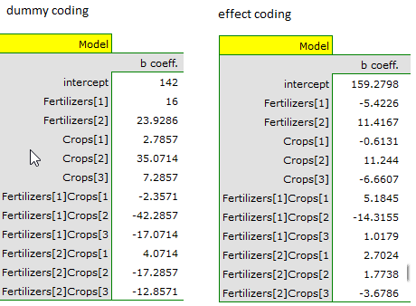
The coefficients of the regression model can be used for prediction via the multiple regression – prediction menu, remembering to code the new data appropriately depending on the model selected.

Checking assumptions
Checking the main assumptions will consist of comparing variances and visually determining the normality of the model residuals.

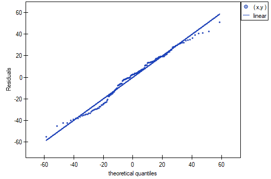
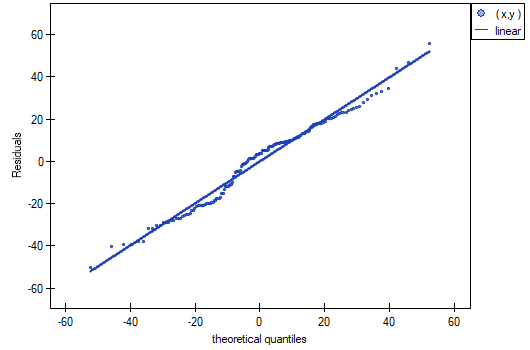
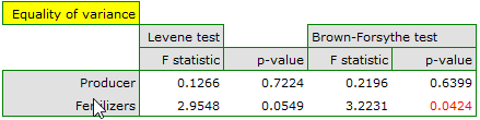
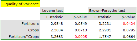
The Q-Q normality plot of the model residuals for the first and second analyses shows the model residuals well distributed around a straight line, indicating a good fit of the residuals to the normal distribution. The comparison of variances is performed using Levene's test or the Brown-Forsythe test. For these tests, we can assume that the results obtained are inconclusive and are on the borderline of equality of variances.

FOR THOSE INTERESTED

Formulas – sums of squares

Type I sums of squares
For example: if we place the factors in the model in the order indicated: \(A\), \(B\), \(A*B\), \(C\), \(A*C\), \(B*C\), \(A*B*C\), \(D\), then the significance for factor \(A*C\) takes the whole model into account (through the sums of squares for the error), but only the factors \(A\), \(B\), \(A*B\), \(C\) are used explicitly as confounding variables. The sums of squares for factor \(A*C\) are then calculated as follows:

\[ SS(A*C)=SS(A, B, A*B, C, A*C, B*C, A*B*C, D)-SS(A, B, A*B, C) \]

Type II sums of squares
For example: if we include the factors \(A\), \(B\), \(A*B\), \(C\), \(A*C\), \(B*C\), \(A*B*C\), \(D\) in the model, then the significance for factor \(A*C\) takes the whole model into account, but the first-order variables \(A\), \(B\), \(C\), \(D\) and all other second-order variables \(A*B\), \(B*C\) are used explicitly as confounding variables. The sums of squares for factor \(A*C\) are then calculated as follows:

\[ SS(A*C)=SS(A, B, A*B, C, A*C, B*C, A*B*C, D)-SS(A, B, A*B, C, B*C, D) \]

Type III sums of squares
For example: if we include the factors \(A\), \(B\), \(A*B\), \(C\), \(A*C\), \(B*C\), \(A*B*C\), \(D\) in the model, then the significance for variable \(A*C\) takes the whole model into account, and all factors except the one under study, i.e. \(A\), \(B\), \(A*B\), \(C\), \(B*C\), \(A*B*C\), \(D\), are used explicitly as confounding variables. The sums of squares for factor \(A*C\) are then calculated as follows:

\[ SS(A*C)=SS(A, B, A*B, C, A*C, B*C, A*B*C, D)-SS(A, B, A*B, C, B*C, A*B*C, D) \]

Hypotheses – ANOVA approach
Hypotheses for factor \(A\):

\[\begin{array}{cl} \mathcal{H}_0: & \mu_1=\mu_2=...=\mu_a,\\ \mathcal{H}_1: & \text{not all }\mu_i\text{ are equal to each other }(i=1,2,...,a), \end{array}\]

where \(\mu_1,\mu_2,...,\mu_a\) – the means of factor \(A\) for its individual categories.

Hypotheses for factor \(B\):

\[\begin{array}{cl} \mathcal{H}_0: & \mu_1=\mu_2=...=\mu_b,\\ \mathcal{H}_1: & \text{not all }\mu_j\text{ are equal to each other }(j=1,2,...,b), \end{array}\]

where \(\mu_1,\mu_2,...,\mu_b\) – the means of factor \(B\) for its individual categories.

Hypotheses for the interaction of factors \(A*B\):

\[\begin{array}{cl} \mathcal{H}_0: & \mu_1=\mu_2=...=\mu_{ab},\\ \mathcal{H}_1: & \text{not all }\mu_k\text{ are equal to each other }(k=1,2,...,ab), \end{array}\]

where \(\mu_1,\mu_2,...,\mu_{ab}\) – the means of the interaction of factors \(A*B\) for their individual categories.

Hypotheses – regression approach
Hypotheses for factor \(A\):

\[\begin{array}{cl} \mathcal{H}_0: & \alpha_1=\alpha_2=...=\alpha_a=0,\\ \mathcal{H}_1: & \text{not all }\alpha_i=0, \end{array}\]

Hypotheses for factor \(B\):

\[\begin{array}{cl} \mathcal{H}_0: & \beta_1=\beta_2=...=\beta_b=0,\\ \mathcal{H}_1: & \text{not all }\beta_j=0, \end{array}\]

Hypotheses for the interaction of factors \(A*B\):

\[\begin{array}{cl} \mathcal{H}_0: & (\alpha\beta)_1=(\alpha\beta)_2=...=(\alpha\beta)_{ab}=0,\\ \mathcal{H}_1: & \text{not all }(\alpha\beta)_k=0, \end{array}\]