 PQStat
The Friedman ANOVA
When to use this test:
The Friedman repeated-measures analysis of variance by ranks (Friedman, 1937[67]) is the non-parametric equivalent of the ANOVA for dependent groups. It is used when measurements of the analysed feature are taken several times on the same objects, and the assumptions of the parametric test are not met – also when we have rankings from different judges and want to assess their agreement. The Iman-Davenport (1980[89]) modification of this statistic is now recommended in place of the traditional Friedman statistic, which tends to be overly conservative.
Assumptions
- measurement on an ordinal scale or an interval scale,
- a dependent model.
When there are gaps in the data, you can instead calculate the Durbin ANOVA (balanced gaps) or the Skillings-Mack ANOVA (gaps in any arrangement). If we are interested in a trend in the arrangement of the studied groups, we can additionally perform the Page test for trend.
How to set up the analysis
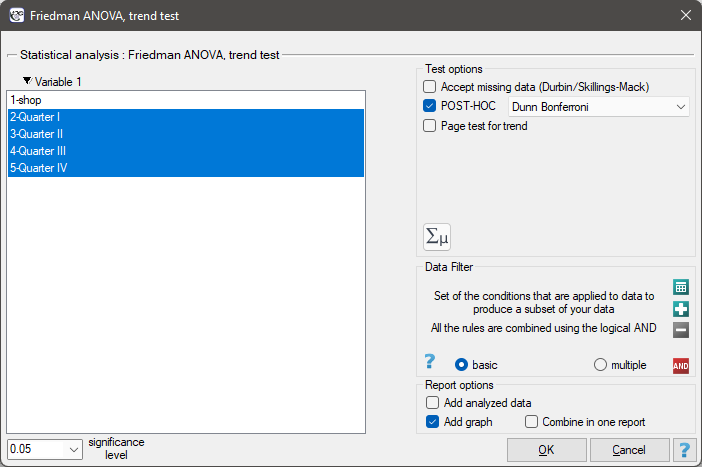
Statistics \(\to\) Nonparametric tests \(\to\) Friedman ANOVA (missing data allowed) (or via the Wizard).
Performing and interpreting the analysis
Example 1. (chocolate bar.pqs file)
Quarterly sales of a certain chocolate bar were measured in 14 randomly chosen supermarkets. The study began in January and ended in December. During the second quarter, an intensive billboard advertising campaign for the product was underway. We will check whether the campaign had an effect on the sales of the advertised chocolate bar.
| Shop | Quarter I | Quarter II | Quarter III | Quarter IV |
| SK1 | 3415 | 4556 | 5772 | 5432 |
| SK2 | 1593 | 1937 | 2242 | 2794 |
| SK3 | 1976 | 2056 | 2240 | 2085 |
| SK4 | 1526 | 1594 | 1644 | 1705 |
| SK5 | 1538 | 1634 | 1866 | 1769 |
| SK6 | 983 | 1086 | 1135 | 1177 |
| SK7 | 1050 | 1209 | 1245 | 977 |
| SK8 | 1861 | 2087 | 2054 | 2018 |
| SK9 | 1714 | 2415 | 2361 | 2424 |
| SK10 | 1320 | 1621 | 1624 | 1551 |
| SK11 | 1276 | 1377 | 1522 | 1412 |
| SK12 | 1263 | 1279 | 1350 | 1490 |
| SK13 | 1271 | 1417 | 1583 | 1513 |
| SK14 | 1436 | 1310 | 1357 | 1468 |
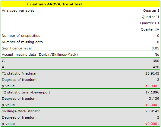
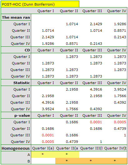
The Dunn POST-HOC analysis with the Bonferroni correction indicates differences in sales between quarters I and III, and between I and IV, while the equivalent analysis using the stronger Conover-Iman test indicates differences between all quarters except III and IV.
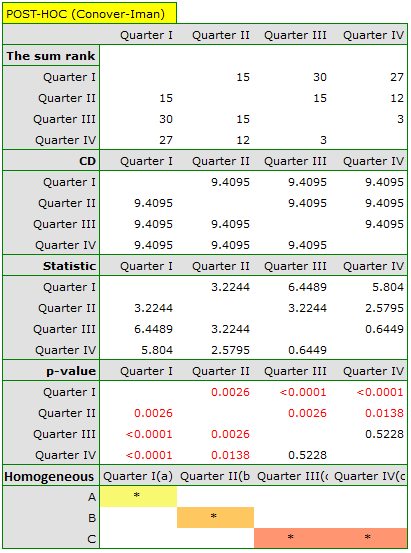
The graph shows the homogeneous groups determined by the Conover-Iman test.
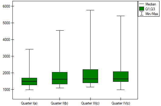
We can provide a detailed description of the data by selecting Descriptive statistics in the analysis window  .
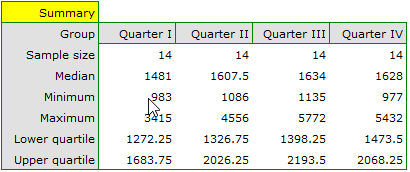
If the data had been described with an ordinal scale with few categories, it would be worth presenting them also as counts and percentages – in this example, however, that would not be a good method of description.
Hypotheses: they relate to the equality of the sum of ranks for successive measurements or are simplified to medians:
where \(\theta_1,\theta_2,...\theta_k\) – medians of the analysed feature at successive measurements in the population studied.
Formulas: two test statistics are determined: the Friedman statistic
and its Iman-Davenport modification
where:
\(n\) – sample size,
\(R_{ij}\) – ranks assigned to successive measurements \((j=1,2,...k)\), separately for each object studied \((i=1,2,...n)\),
\(\displaystyle C=1-\frac{\sum(t^3-t)}{n(k^3-k)}\) – correction for ties,
\(t\) – number of cases included in a tie. The correction \(C\) is used when ties occur (otherwise \(C=1\)).
The \(T_1\) statistic asymptotically (for large sample sizes) has the \(\chi^2\) distribution with \(df=k-1\) degrees of freedom. The \(T_2\) statistic has the F Snedecor distribution with \(df_1=k-1\) and \(df_2=(n_j-1)(k-1)\) degrees of freedom.
The \(p\) value, determined on the basis of the test statistic, is compared with \(\alpha\): if \(p \le \alpha\), we reject \(\mathcal{H}_0\) in favor of \(\mathcal{H}_1\); if \(p > \alpha\), there is no reason to reject \(\mathcal{H}_0\).
POST-HOC tests
An introduction to contrasts and POST-HOC tests is provided in section Contrasts and POST-HOC tests, which concerns the one-way analysis of variance.
The Dunn test
Used for simple comparisons (the counts in each measurement are always the same). The Dunn test (Dunn, 1964[53]) is corrected for multiple testing – most often with the Bonferroni or Sidak correction (other, newer corrections are described in more detail in the Multiple comparisons section).
- \(\mathfrak{(i)}\)
The critical difference is calculated using the formula:
\[ CD=Z_{\alpha(corrected)}\sqrt{\frac{k(k+1)}{6n}}, \]where \(Z_{\alpha(corrected)}\) is the critical value (statistic) of the normal distribution for the significance level \(\alpha\) adjusted for the number of possible simple comparisons \(c\) according to the selected correction.
- \(\mathfrak{(ii)}\)
The test statistic is defined by:
\[ Z=\frac{\sum_{j=1}^k c_j\overline{R}_j}{\sqrt{\frac{k(k+1)}{6n}}}, \]where \(\overline{R}_j\) – mean rank of measurement \(j\), for \((j=1,2,...k)\). The test statistic asymptotically (for large sample sizes) has the normal distribution, and the \(p\) value is adjusted for the number of possible simple comparisons according to the selected correction.
The Conover-Inman test
The non-parametric equivalent of LSD Fisher[48], used for simple comparisons (the counts in each measurement are always the same).
- \(\mathfrak{(i)}\)
The critical difference is calculated using the formula:
\[ CD=\sqrt{F_{\alpha,1,df_2}}\cdot\sqrt{\frac{2\left(n_jA-\sum_{j=1}^tR_j^k\right)}{(n_j-1)(k-1)}}, \]where \(\displaystyle A=\sum_{i=1}^{n_j}\sum_{j=1}^kR_{ij}^2\) – sum of squared ranks, and \(F_{\alpha,1,df_2}\) is the critical value (statistic) of the F Snedecor distribution for a given significance level \(\alpha\) and for degrees of freedom 1 and \(df_2\), respectively.
- \(\mathfrak{(ii)}\)
The test statistic is defined by:
\[ t=\frac{\sum_{j=1}^k c_jR_j}{\sqrt{\frac{2\left(n_jA-\sum_{j=1}^tR_j^k\right)}{(n_j-1)(k-1)}}}, \]where \(R_j\) – sum of ranks of measurement \(j\), for \((j=1,2,...k)\). The test statistic has the \(t\)-Student distribution with \(df_2\) degrees of freedom.