The single-sample t-test

The single-sample \(t\)-test

When to use this test:

The single-sample \(t\)-test (single-sample \(t\) test) lets you verify the hypothesis that the sample studied, with mean \(\overline{x}\), comes from a population for which the mean \(\mu\) is a given value.

Assumptions

measurement on an interval scale,
normality of distribution of the feature studied.

Note! When the sample is large and the population standard deviation is known, the test statistic can be calculated using the formula \(t=\frac{\overline{x}-\mu_0}{\sigma}\sqrt n\), which then has the normal distribution. As \(n \rightarrow \infty\), the \(t\)-Student distribution converges to the normal distribution \(N(0,1)\) – in practice, it is assumed that for \(n>30\) the \(t\)-Student distribution can be approximated by the normal distribution. Calculations can be based on raw records or on averaged data, i.e. the arithmetic mean, standard deviation, and sample size.

Definitions of measures

Cohen's d – a standardised effect size that determines how large a part of the variability present is accounted for by the difference between the means. When interpreting an effect, researchers often use general guidelines defined by Cohen[47], defining a small (0.2), medium (0.5), and large (0.8) effect size.

How to set up the analysis

Statistics \(\to\) Parametric tests \(\to\) t-Student (or via the Wizard).

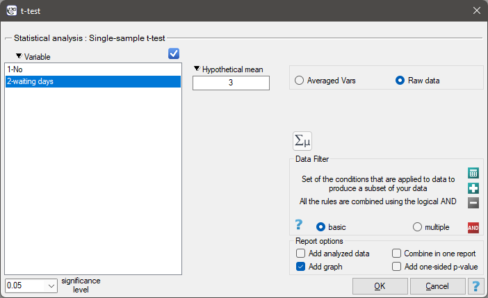
Performing and interpreting the analysis

Example 1. (courier.pqs file)
We want to check whether the waiting time for a delivery by a certain courier company is, on average, 3 days (\(\mu_0=3\)). To do this, a sample of 22 people was drawn from the population of the company's customers, and the number of days that elapsed between sending the parcel and its delivery was recorded for each. The following values were obtained: (1, 1, 1, 2, 2, 2, 2, 3, 3, 3, 4, 4, 4, 4, 4, 5, 5, 6, 6, 6, 7, 7).

The number of days of waiting for a delivery in the population studied satisfies the assumption of normality of distribution.

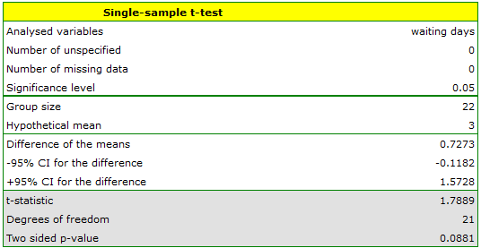
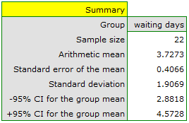
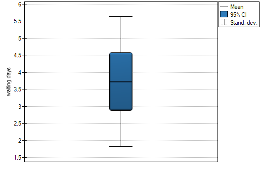
\(p=0.088074\) (not statistically significant, \(\alpha=0.05\))

There is no reason to reject the null hypothesis that the mean number of days of waiting for a delivery by the courier company analysed is 3.

For the sample studied, the mean is \(\overline{x}=3.727\), and the standard deviation is \(sd=1.907\).

FOR THOSE INTERESTED

Hypotheses:

\(\begin{array}{cc} \mathcal{H}_0: & \mu=\mu_0,\\ \mathcal{H}_1: & \mu\ne \mu_0, \end{array}\)

where:
\(\mu\) – the mean of the feature in the population represented by the sample,
\(\mu_0\) – a given value.

Formulas:

The test statistic is defined by:

\[ t=\frac{\overline{x}-\mu_0}{sd}\sqrt{n}, \]

where:
\(sd\) – the sample standard deviation,
\(n\) – the sample size.

The test statistic has the \(t\)-Student distribution with \(n-1\) degrees of freedom.

The \(p\) value, determined on the basis of the test statistic, is compared with the significance level \(\alpha\): if \(p \le \alpha\), we reject \(\mathcal{H}_0\) in favor of \(\mathcal{H}_1\); if \(p > \alpha\), there is no reason to reject \(\mathcal{H}_0\).

Cohen's d

\[ d=\left|\frac{\overline{x}-\mu_0}{sd}\right| \]