 PQStat
The Jonckheere-Terpstra test for trend
When to use this test:
The Jonckheere-Terpstra test for trend, described independently by Jonckheere (1954)[92] and Terpstra (1952)[163], can be performed in the same situation as the Kruskal-Wallis ANOVA, since it is based on the same assumptions. Unlike the Kruskal-Wallis ANOVA, however, it does not check for arbitrary differences between groups, but whether the medians of successive, ordered populations increase or decrease in the expected direction.
Assumptions
- measurement on an ordinal scale or an interval scale,
- an independent model,
- a known or assumed order of the compared populations.
How to set up the analysis
Statistics \(\to\) Nonparametric tests \(\to\) Kruskal-Wallis ANOVA (or via the Wizard).
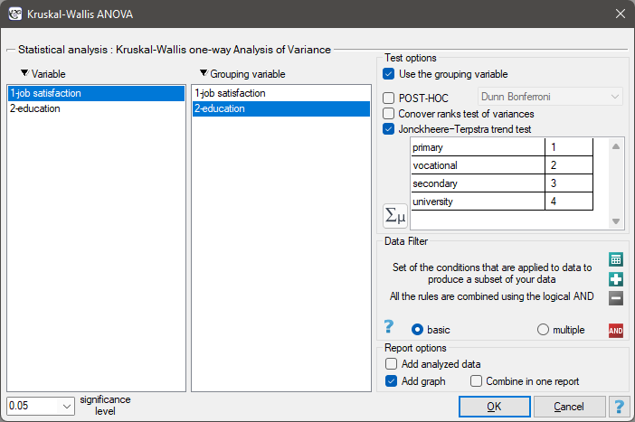
 button.
Performing and interpreting the analysis
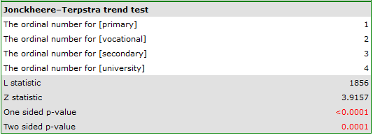
Continuation of Example 1 (jobSatisfaction.pqs file): it is suspected that better-educated people have higher job demands, which may reduce satisfaction with their first job, which often does not meet such demands. We will therefore check whether the level of satisfaction with the first job changes in the expected direction with the level of education.
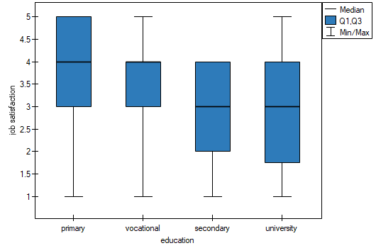
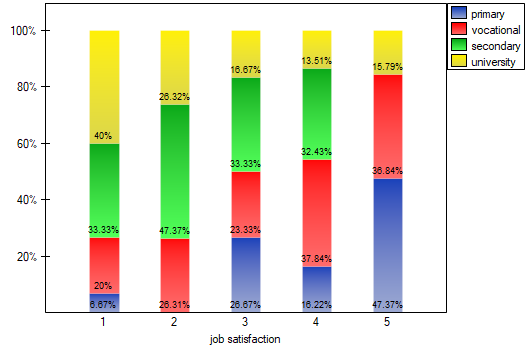
We can also confirm the existence of this trend by showing the percentage distribution of the responses obtained.
Hypotheses (simplified to medians):
Formulas: The test statistic is defined by:
where:
\(L\) – sum of the \(l_{ij}\) values obtained for each pair of compared populations,
\(l_{ij}\) – number of results higher than a given value in the next group,
\(SE=\sqrt{\frac{A}{72}+\frac{B}{36N(N-1)(N-2)}+\frac{C}{8N(N-1)}}\),
\(A=N(N-1)(2N+5)-\sum_{j=1}^kn_j(n_j-1)(2n_j+5)-\sum_{l=1}^gt_l(t_l-1)(2t_l+5)\),
\(B=\sum_{j=1}^kn_j(n_j-1)(n_j-2)\cdot\sum_{l=1}^gt_l(t_l-1)(t_l-2)\),
\(C=\sum_{j=1}^kn_j(n_j-1)\cdot\sum_{l=1}^gt_l(t_l-1)\),
\(g\) – number of groups of different tied ranks,
\(t_l\) – number of cases included in a tie,
\(N=\sum_{j=1}^k n_j\),
\(n_j\) – sample sizes for \((j=1,2,...k)\).
Interpretation: The formula for the test statistic \(Z\) includes a correction for tied ranks. This correction is applied when tied ranks are present (when there are no tied ranks, the formula reduces to the original Jonckheere-Terpstra formula without this correction). The \(Z\) statistic asymptotically (for large sample sizes) has the normal distribution.
With the expected direction of the trend known, the alternative hypothesis is one-sided and the one-sided \(p\) value is interpreted. Interpreting the two-sided \(p\) value means that the researcher does not know (does not assume) the direction of the possible trend.
The \(p\) value, determined on the basis of the test statistic, is compared with \(\alpha\): if \(p \le \alpha\), we reject \(\mathcal{H}_0\) in favor of \(\mathcal{H}_1\); if \(p > \alpha\), there is no reason to reject \(\mathcal{H}_0\).