 PQStat
The ROC curve
When to use:
A diagnostic test is used to distinguish objects with a given feature (marked as (+), e.g. ill people) from objects without the feature (marked as (–), e.g. healthy people). For a diagnostic test to be considered valuable, it should yield a relatively small number of misclassifications. If the test is based on a dichotomous variable, the proper tool for evaluating its quality is the analysis of a \(2\times2\) contingency table. Most often, however, diagnostic tests are based on continuous variables or variables with ordered categories. In such a situation, the proper means of evaluating a test's ability to distinguish (+) from (–) are ROC curves (Receiver Operating Characteristic).
It is often observed that as the value of the diagnostic variable increases, the odds of the phenomenon studied occurring increase too, or the other way round: as the value of the diagnostic variable increases, the odds of the phenomenon studied occurring decrease. In such cases, ROC curves are used to choose the optimal cut-off point, i.e. a value of the diagnostic variable that best divides the population studied into two groups: (+), in which the phenomenon occurs, and (–), in which it does not. When two or more ROC curves are built on the basis of studies carried out on the same objects, these curves can be compared in terms of classification quality.
Assumptions
Definitions of measures
Let us assume we have at our disposal a sample of \(n\) elements, in which each object obtains one of \(k\) values of the diagnostic variable. Each of the values obtained for the diagnostic variable, \(x_1, x_2, ...x_k\), becomes a potential cut-off \(x_{cat}\). If the diagnostic variable is a:
- stimulant (as its value increases, the odds of the phenomenon studied occurring increase), then values greater than or equal to the cut-off (\(x_i\geq x_{cat}\)) are classified into group (+);
- destimulant (as its value increases, the odds of the phenomenon studied occurring decrease), then values less than or equal to the cut-off (\(x_i\leq x_{cat}\)) are classified into group (+).
For each of the \(k\) cut-offs, we determine the true positive (TP), true negative (TN), false positive (FP), and false negative (FN) values, and on their basis sensitivity, specificity, and the remaining measures described in the Evaluation of a diagnostic test section.
\(AUC\) (area under curve) – the size of the area under the ROC curve, which lies in the range \(\langle0;1\rangle\). The ROC curve is built from the sensitivity and specificity values determined for successive cut-offs – the abscissa axis represents \(x=1-\)specificity, and the ordinate axis \(y=\)sensitivity, and the resulting points are joined together.
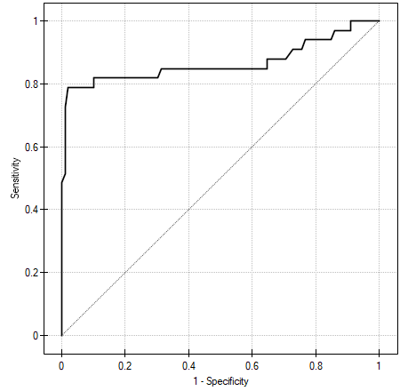
The greater the \(AUC\), the more accurately we can classify objects into group (+) and group (–) on the basis of the diagnostic variable analysed, and so the more effectively that diagnostic variable can be used as a classifier. When the ROC curve coincides with the diagonal \(y=x\) (i.e. \(AUC=0.5\)), the decision made on the basis of the diagnostic variable is exactly as good as a random split of the objects studied into groups (+) and (–).
The area \(AUC\), the error \(SE_{AUC}\), and the confidence interval for \(AUC\) are calculated on the basis of:
- \(\star\) the nonparametric DeLong method (DeLong E.R. et al., 1988[52]; Hanley J.A. and Hajian-Tilaki K.O., 1997[76]) – recommended,
- \(\star\) the nonparametric Hanley-McNeil method (Hanley J.A. and McNeil M.D., 1982[77]),
- \(\star\) the Hanley-McNeil method assuming a bi-negative exponential distribution (Hanley J.A. and McNeil M.D., 1982[77]) – calculated only when groups (+) and (–) are equal in size.
Performing and interpreting the analysis
The \(AUC\) significance test is always performed together with the selection of the optimal cut-off – see Example 1 in the next section.
For the classification to be better than a random split of the objects into two classes, the area under the ROC curve should be significantly greater than the area under the line \(y=x\), i.e. than 0.5.
Hypotheses:
\(\begin{array}{cl} \mathcal{H}_0: & AUC=0.5, \\ \mathcal{H}_1: & AUC\neq 0.5. \end{array}\)
Formulas:
The test statistic is defined by:
where:
\(SE_{0.5}=\sqrt{\frac{n_{(+)}+n_{(-)}+1}{12n_{(+)}n_{(-)}}}\),
\(n_{(+)}\) – the size of group (+), in which the phenomenon studied genuinely occurs,
\(n_{(-)}\) – the size of group (–), in which the phenomenon studied genuinely does not occur.
The \(Z\) statistic asymptotically (for large sample sizes) has the normal distribution.
The \(p\) value, determined on the basis of the test statistic, is compared with the significance level \(\alpha\): if \(p \le \alpha\), we reject \(\mathcal{H}_0\) in favor of \(\mathcal{H}_1\); if \(p > \alpha\), there is no reason to reject \(\mathcal{H}_0\).
Additionally, once we assume that the diagnostic parameter yields a high \(AUC\), we can select the optimal cut-off.
Revised predictive values
The PQStat program calculates the prevalence on the basis of the sample available. The calculated prevalence will reflect the occurrence of the phenomenon studied (disease) in the population when the study is a screening study covering a large sample representative of the population. When only people suspected of the disease are referred for testing, the prevalence calculated for them may be considerably higher than the prevalence in the population. Since both the positive and negative predictive values depend on the prevalence, if we know this coefficient a priori for the population, we can use it to calculate, for each cut-off \(x_{cat}\), revised predictive values according to Bayes's formulas:
where \(P_{a priori}\) – the prevalence specified by the user, the so-called pre-test probability of disease.
Summary:
The measures determined for each cut-off are gathered in a table:
| \(x_{cat}\) | sensitivity | specificity | \(\textbf{PPV}\) | \(\textbf{NPV}\) | \(\textbf{LR}_+\) | \(\textbf{LR}_-\) | \(\textbf{Acc}\) | \(\textbf{PPV}_{rev}\) | \(\textbf{NPV}_{rev}\) |
| \(x_1\) | sensitivity\(_1\) | specificity\(_1\) | \(PPV_1\) | \(NPV_1\) | \(LR_{+1}\) | \(LR_{-1}\) | \(Acc_1\) | \(PPV_{rev1}\) | \(NPV_{rev1}\) |
| \(x_2\) | sensitivity\(_2\) | specificity\(_2\) | \(PPV_2\) | \(NPV_2\) | \(LR_{+2}\) | \(LR_{-2}\) | \(Acc_2\) | \(PPV_{rev2}\) | \(NPV_{rev2}\) |
| ⋮ | ⋮ | ⋮ | ⋮ | ⋮ | ⋮ | ⋮ | ⋮ | ⋮ | ⋮ |
| \(x_k\) | sensitivity\(_k\) | specificity\(_k\) | \(PPV_k\) | \(NPV_k\) | \(LR_{+k}\) | \(LR_{-k}\) | \(Acc_k\) | \(PPV_{revk}\) | \(NPV_{revk}\) |
Selection of the optimal cut-off
When to use:
The point sought is a certain value of the diagnostic variable that optimally divides the population studied into two groups: (+), in which the phenomenon occurs, and (–), in which it does not. Choosing the optimal cut-off is not easy, since it requires specialist knowledge of the subject of the study. For example, a different cut-off will be needed for a test used in screening studies covering a large group of people, e.g. in a mammography study, than in invasive studies conducted to confirm an earlier suspicion, e.g. in histopathology. Using advanced mathematical tools, we can find such a point, the so-called cut-off, that is most favourable from a mathematical point of view.
Definitions of measures
The PQStat program allows the optimal cut-off to be selected using:
The tangent method (cost index) – calculated on the basis of sensitivity, specificity, the costs of wrong decisions, and the prevalence. The errors that can be made when assigning the objects studied to group (+) and group (–) are false positive results (\(FP\)) and false negative results (\(FN\)). If making these errors is equally costly (ethical, financial, etc. costs), then in the cost FP field and the cost FN field we enter the same positive value – usually 1. If, on the other hand, we judge that one type of error carries a greater cost than the other, we assign it a correspondingly greater weight. The optimal cut-off value is calculated using \(m\) – the slope of the tangent to the ROC curve, defined with reference to the costs of wrong decisions and the prevalence.
Youden's index – conceptually, this is the maximum distance between the line forming the diagonal of a unit square and a point on the ROC curve[180].
Distance to the top-left corner – conceptually, this is the minimum distance between the top-left corner of a unit square (i.e. the point at which sensitivity and specificity can be highest) and a point on the ROC curve.
Costs graph – shows the calculated values of a wrong diagnosis together with their costs. The point marked on the graph is the minimum of the cost function.
Sensitivity and specificity intersection graph – lets you locate the point at which the values of sensitivity and specificity are simultaneously greatest.
How to set up the analysis
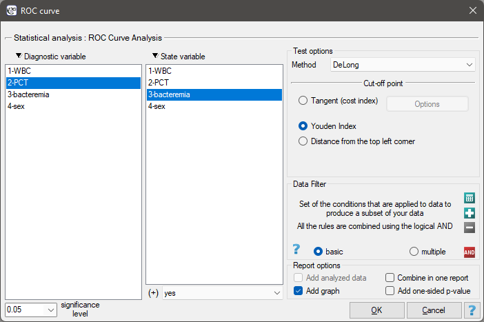
Advanced statistics \(\to\) Diagnostic tests \(\to\) ROC curve.
Performing and interpreting the analysis
Example 1. (bacteremia.pqs file)
Persistent high fever in an infant or young child without a clear, established cause is an indication for testing for bacteremia. The parameters considered most useful and reliable for screening and monitoring bacterial infections are:
- WBC – white blood cell count,
- PCT – procalcitonin.
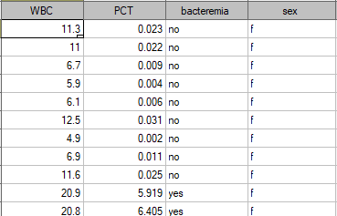
It is assumed that in a healthy infant or young child, WBC should not exceed 15 thousand/µl, and PCT should be below 0.5 ng/ml. Example values of these indicators for 136 children up to 3 years of age with persistent fever \(>39^0C\) are shown in the table excerpt below:
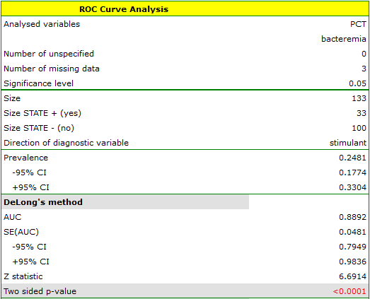
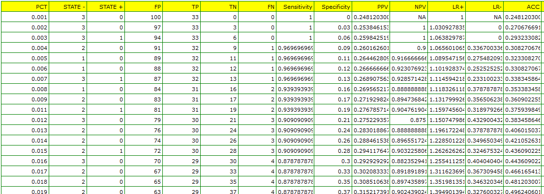
One possible way of analysing the PCT indicator is to convert it into a dichotomous variable by choosing a cut-off (e.g. \(x_{cat}=0.5\) ng/ml), above which the test is considered “positive”. How good this split is will be shown by the sensitivity and specificity values. We want, however, to use a more comprehensive approach – that is, to calculate sensitivity and specificity not just for a single value, but for every PCT value obtained in the sample – in other words, to build a ROC curve. On the basis of the information obtained this way, we want to check whether the PCT indicator is genuinely useful for diagnosing bacteremia, and if so, what the optimal cut-off is, above which we can consider the test “positive”– detecting bacteremia.
Since bacteremia is accompanied by an elevated PCT level, we treat this indicator as a stimulant. In the state variable, we must specify which value in the bacteremia column indicates its presence – here we select the value “yes”. In the report, besides the result of the statistical test, we can find a detailed description of every possible cut-off.
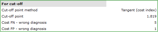
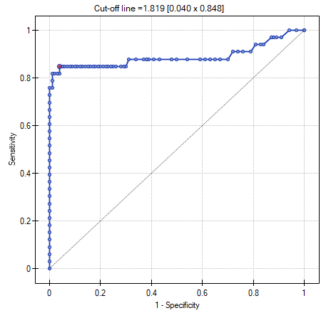
We therefore return to the analysis (the  button) to determine the optimal cut-off. The algorithm for finding the optimal cut-off takes into account the costs of wrong decisions and the prevalence:
- (1) FN cost – wrong diagnosis is the cost of concluding that the patient does not have bacteremia when they genuinely do (the cost of a false negative decision);
- (2) FP cost – wrong diagnosis is the cost of concluding that the patient has bacteremia when they genuinely do not (the cost of a false positive decision).
Since FN costs are much more serious than FP costs, we enter a greater value in the first field than in the second – we decided this would be 5. The PCT value is to be used in screening studies, so we do not provide the population prevalence (the a priori prevalence), which is very low, but instead keep the prevalence estimated from the sample. We do this so as not to move the PCT cut-off too high and increase the number of false negative results.
Another way of choosing the cut-off is to analyse the costs graph and the sensitivity-specificity intersection graph:
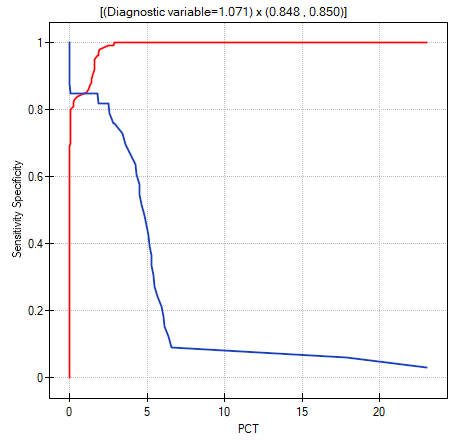
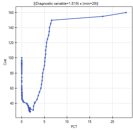
The costs graph shows that the minimum cost of wrong decisions falls at PCT=1.819. The sensitivity and specificity values, on the other hand, are similar at PCT=1.071.
The tangent method (cost index)
The optimal cut-off is taken to be the value of the diagnostic variable at which the expression:
reaches its minimum (Zweig M.H., 1993[186]). The slope angle \(m\) is defined with reference to the costs of wrong decisions and the prevalence. By default, the costs of wrong decisions equal 1, and the prevalence is estimated from the sample. Knowing the prevalence a priori (\(P_{a priori}\)) and the costs of wrong decisions, the user can influence the value of \(m\), and thereby the search for the optimal cut-off.
Youden's index
Distance to the top-left corner
Costs graph
The values of a wrong diagnosis are calculated according to the formula:
ROC curves comparison
When to use:
Very often the aim of a study is to compare the size of the area under one ROC curve (\(AUC_1\)) with the area under another ROC curve (\(AUC_2\)). A ROC curve with a larger area usually allows more accurate classification of objects. The methods used to compare the areas depend on the study model.
Assumptions
- dependent model – the ROC curves compared are built from measurements made on the same objects,
- independent model – the ROC curves compared are built from measurements made on different objects.
How to set up the analysis
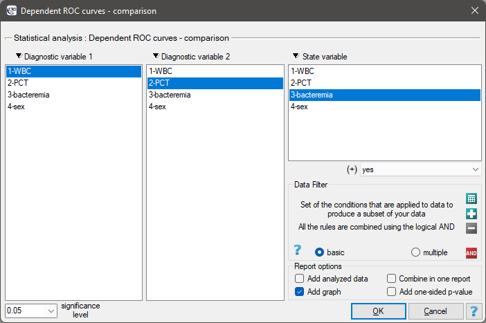
For the dependent model: Advanced statistics \(\to\) Diagnostic tests \(\to\) Dependent ROC Curves – comparison.
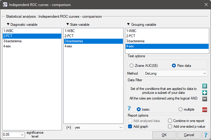
For the independent model: Advanced statistics \(\to\) Diagnostic tests \(\to\) Independent ROC Curves – comparison.
Performing and interpreting the analysis
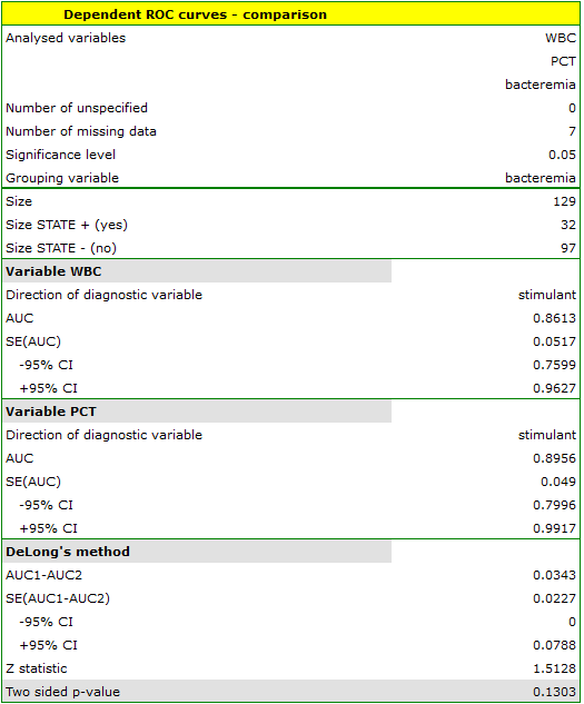
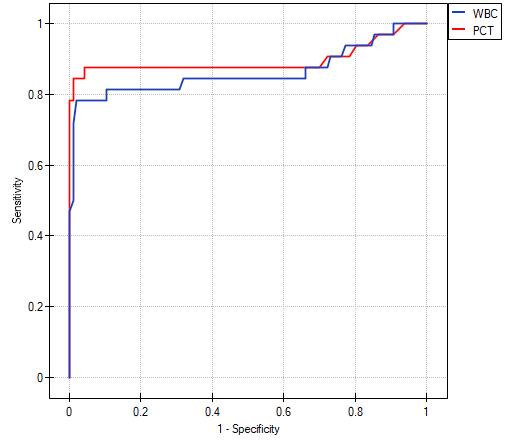
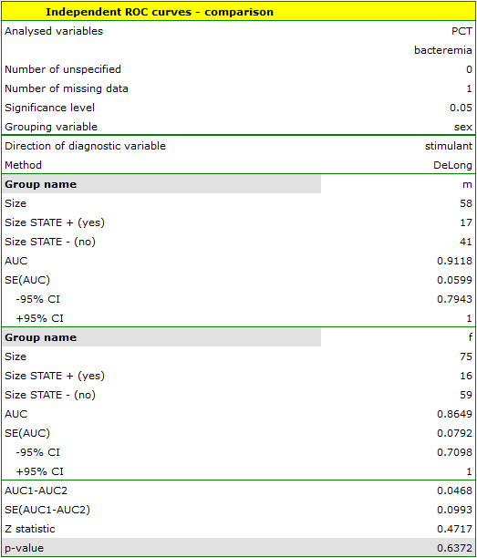
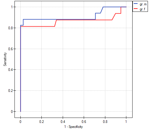
Continuation of Example 1 (bacteremia.pqs file): we will perform 2 comparisons – (1) we will build 2 ROC curves to compare the diagnostic value of the WBC and PCT parameters (dependent model – the same children); (2) we will build 2 ROC curves to compare the diagnostic value of the PCT parameter for boys and girls (independent model – different children).
(1) WBC vs PCT (dependent model)
Both WBC and PCT are stimulants (high values of these parameters accompany bacteremia).
(2) PCT: girls vs boys (independent model)
The PCT parameter is a stimulant (its high values accompany bacteremia); we compare its diagnostic value separately for girls and boys.
Hypotheses (common to both models):
\(\begin{array}{cl} \mathcal{H}_0: & AUC_1=AUC_2, \\ \mathcal{H}_1: & AUC_1\neq AUC_2. \end{array}\)
Dependent model
The test statistic is defined by:
where \(AUC_1\), \(AUC_2\), and the standard error of the difference in areas \(SE_{AUC_1-AUC_2}\) are calculated on the basis of the nonparametric method proposed by DeLong (DeLong E.R. et al., 1988[52]; Hanley J.A. and Hajian-Tilaki K.O., 1997[76]).
The \(Z\) statistic asymptotically (for large sample sizes) has the normal distribution.
Independent model
The test statistic (Hanley J.A. and McNeil M.D., 1983[78]) is defined by:
where \(AUC_1\), \(AUC_2\), and the standard errors of the areas \(SE_{AUC_1}\), \(SE_{AUC_2}\) are calculated on the basis of:
- \(\star\) the nonparametric DeLong method (DeLong E.R. et al., 1988[52]; Hanley J.A. and Hajian-Tilaki K.O., 1997[76]) – recommended,
- \(\star\) the nonparametric Hanley-McNeil method (Hanley J.A. and McNeil M.D., 1982[77]).
The \(Z\) statistic asymptotically (for large sample sizes) has the normal distribution.
For both models: the \(p\) value, determined on the basis of the test statistic, is compared with the significance level \(\alpha\): if \(p \le \alpha\), we reject \(\mathcal{H}_0\) in favor of \(\mathcal{H}_1\); if \(p > \alpha\), there is no reason to reject \(\mathcal{H}_0\).