 PQStat
Hotelling's analysis, proposed by Hotelling (1931)[85] (1947)[86] and Mahalanobis (1930[111], 1936[112]), extends the \(t\)-Student tests to the domain of multiple variables. As a result, we can subject many different features of the objects studied to simultaneous analysis.
Hotelling's T-square test for a single sample
When to use this test:
This test lets you check whether \(k\) variables in the population studied, \(X_1,X_2,...,X_k\), are characterised by the means specified by the researcher – it is a multivariate extension of the single-sample \(t\)-test.
Assumptions
- measurement on an interval scale,
- a multivariate normal distribution, or normality of distribution of each variable studied.
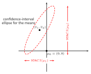
Example – interpreting the Hotelling test ellipse for two variables
The given point described by the mean values (\(\mu_0=(0,0)\)) lies outside the ellipse, which means that Hotelling's test rejects \(\mathcal{H}_0\), but with the univariate approach (confidence intervals for each variable separately) we are unable to reject \(\mathcal{H}_0\) and thus cannot identify the variable the difference concerns.
How to set up the analysis
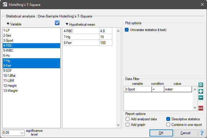
Statistics \(\to\) Parametric tests \(\to\) T-square Hotelling.
Performing and interpreting the analysis
Example 1. (sport.pqs file)
A group of athletes was studied to obtain, among other things, information on health parameters such as:
RBC – red blood cell count,
Hg – haemoglobin [g/dl],
Ferr – ferritin [µg/l].
We want to know how close to the values expected by the researchers are the average levels of RBC, haemoglobin, and ferritin for athletes practising so-called “water”sports. The expected means are:
RBC = 4.8,
Hg = 15 [g/dl],
Ferr = 100 [µg/l].
Since the data sheet contains information on the parameters studied for a larger group of athletes, in the analysis window we select the people practising water sports using a data filter.
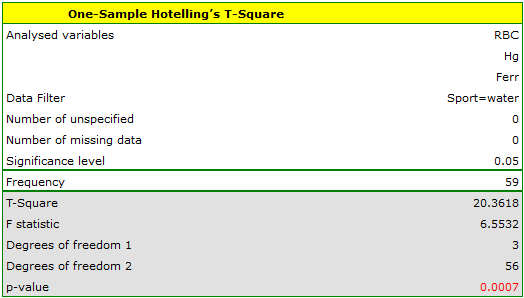
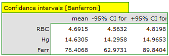
We can look for the differences in the calculated simultaneous confidence intervals or in the intervals with the Bonferroni correction. For ferritin, the simultaneous 95% confidence interval lies below the specified value, indicating a lower population value of ferritin than that specified by the researchers. The intervals for RBC and haemoglobin contain the specified values, which indicates no statistically significant differences.
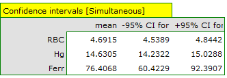
Somewhat narrower intervals are obtained using the Bonferroni correction – in that case not only the interval for ferritin but also the interval for haemoglobin lies below the specified value.
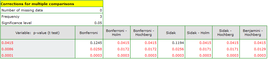
Because of its simplicity, the univariate approach is the one most often used. Here we can choose less conservative multiple-comparison corrections than the Bonferroni or Sidak correction, obtaining in this way differences for all the parameters studied. To adjust the \(p\) values of the \(t\)-Student test, copy those values into a single column of a new data sheet and, from the Statistics menu, choose Correction for multiple comparisons.

Hypotheses:
where:
\(\mu=(\mu_1, \mu_2,..., \mu_k)\) – means of the variables in the population represented by the sample,
\(\mu_0=(\mu_{01}, \mu_{02},..., \mu_{0k})\) – mean values specified by the researcher.
Formulas: The test statistic is defined by:
where:
\(n=n_1=n_2=...=n_k\) – the sample sizes of the individual variables,
\(T^2 = n(\overline{x}-\mu_0)^TS^{-1}(\overline{x}-\mu_0)\) – the original Hotelling test statistic, which has the \(\chi^2\) distribution (recommended for samples with large sizes),
\(\overline{x}=(\overline{x}_1, \overline{x}_2,..., \overline{x}_k)\) – means of the variables in the sample,
\(S\) – the covariance matrix.
The test statistic has the F Snedecor distribution with \(k\) and \(n-k\) degrees of freedom.
The \(p\) value, determined on the basis of the test statistic, is compared with the significance level \(\alpha\): if \(p \le \alpha\), we reject \(\mathcal{H}_0\) in favor of \(\mathcal{H}_1\); if \(p > \alpha\), there is no reason to reject \(\mathcal{H}_0\).
Simultaneous confidence intervals
When, after performing the analysis, we look for the variables the differences concern, we calculate simultaneous confidence intervals for the means:
or the intervals with the Bonferroni correction, to check whether the specified value falls within them. If the specified value falls within the calculated interval, this means the true mean of that variable may actually equal the specified value. When using this method, however, keep in mind that the resulting intervals do not take into account the interrelationships between the individual variables (which Hotelling's test does take into account), only the effect of multiple testing.
When looking for the variables the differences concern, we can also use a univariate approach, performing separate comparisons for each variable with the single-sample \(t\)-test. Unfortunately, this does not account for the interrelationships between variables, but the \(p\) values obtained from the \(t\)-Student test can be adjusted in the Multiple comparisons section.
Hotelling's T-square test for dependent groups
When to use this test:
Used when \(k\) variables under study are measured twice, under different conditions (assuming that the variances of the variables are close to each other in both measurements). If we denote the first measurement by \(X_1,X_2,...,X_k\) and the second by \(Y_1,Y_2,...,Y_k\), we test the hypothesis that the population means of the variables from the first measurement are the same as from the second measurement.
Assumptions
- measurement on an interval scale,
- a multivariate normal distribution, or normality of distribution of each variable studied,
- a dependent model.
How to set up the analysis
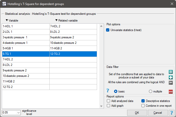
Statistics \(\to\) Parametric tests \(\to\) T-square Hotelling for dependent groups.
Performing and interpreting the analysis
Example 2. (hypertension.pqs file)
In a group of people suffering from hypertension, the effect of treatment on changes in indicators such as: HDL and LDL cholesterol, haemoglobin (HGB), triglycerides (TG), and systolic and diastolic blood pressure was studied. Measurements from 44 patients were taken twice (before treatment and after 3 months of treatment). The resulting values were then compared.
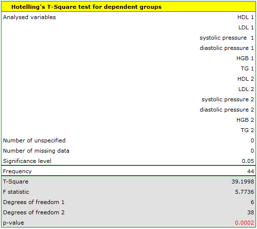
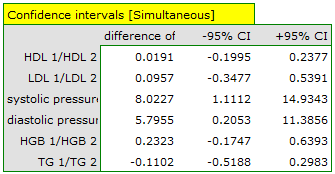
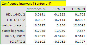
The confidence intervals for systolic and diastolic blood pressure lie above the value 0, indicating a significant decrease in these parameters as a result of treatment. The intervals for the remaining parameters contain the value 0, so we have no evidence of a change resulting from treatment.
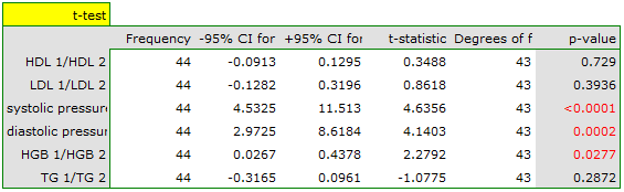
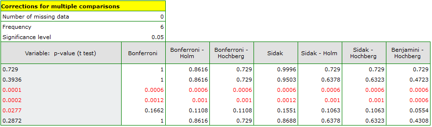
Because of its simplicity, the univariate approach is the one most often used. Using this approach together with a multiple-comparison correction, we likewise conclude that the differences concern only the blood-pressure values. To adjust the \(p\) values of the \(t\)-Student test, copy those values into a single column of a new data sheet and, from the Statistics menu, choose Correction for multiple comparisons.
Definition: equivalently, if we calculate the differences between the pairs of measurements \(d_1, d_2, ..., d_k\), the hypothesis states that the means of the differences in the population studied equal 0.
Hypotheses:
where \(\mu_0=(\mu_{01}, \mu_{02},..., \mu_{0k})\) – the population means of the differences between the first and second measurement.
Formulas: The test statistic is defined by:
where:
\(n=n_1=n_2=...=n_k\) – the sample sizes of the individual differences,
\(T^2 = n(\overline{x}-\overline{y})^TS^{-1}(\overline{x}-\overline{y})\) – the original Hotelling test statistic, which has the \(\chi^2\) distribution (recommended for samples with large sizes),
\(\overline{x}=(\overline{x}_1, \overline{x}_2,..., \overline{x}_k)\) – means of the variables in the sample for the first measurement,
\(\overline{y}=(\overline{y}_1, \overline{y}_2,..., \overline{y}_k)\) – means of the variables in the sample for the second measurement,
\(S\) – the covariance matrix of the differences between the first and second measurement.
The test statistic has the F Snedecor distribution with \(k\) and \(n-k\) degrees of freedom.
The \(p\) value, determined on the basis of the test statistic, is compared with the significance level \(\alpha\): if \(p \le \alpha\), we reject \(\mathcal{H}_0\) in favor of \(\mathcal{H}_1\); if \(p > \alpha\), there is no reason to reject \(\mathcal{H}_0\).
Simultaneous confidence intervals
When, after performing the analysis, we look for the variables the differences concern, we calculate simultaneous confidence intervals for the mean differences:
or the intervals with the Bonferroni correction, to check whether the value 0 falls within them. If the difference can equal 0, this means the difference between the values studied may not actually exist. When using this method, keep in mind that the resulting intervals do not take into account the interrelationships between the variables (which Hotelling's test does take into account), only the effect of multiple testing.
When looking for the variables the differences concern, we can also use a univariate approach, performing separate comparisons for each variable with the \(t\)-test for dependent groups. Unfortunately, this does not account for the interrelationships between variables, but the \(p\) values obtained from the \(t\)-Student test can be adjusted in the Multiple comparisons section.
Hotelling's T-square test for independent groups
When to use this test:
This test lets you check the equality of the means of \(k\) variables studied, \(X_1,X_2,...,X_k\), from the first population, and the means of the same \(k\) variables, \(Y_1,Y_2,...,Y_k\), from the second population.
Assumptions
- measurement on an interval scale,
- a multivariate normal distribution in both populations, or normality of distribution of each variable studied in both populations,
- an independent model,
- equality of variances of the variables studied in both populations, or equality of the covariance matrices – a condition that is especially important for groups of different sizes; when it is not met, a correction should be calculated.
How to set up the analysis
Statistics \(\to\) Parametric tests \(\to\) T-square Hotelling for independent groups.
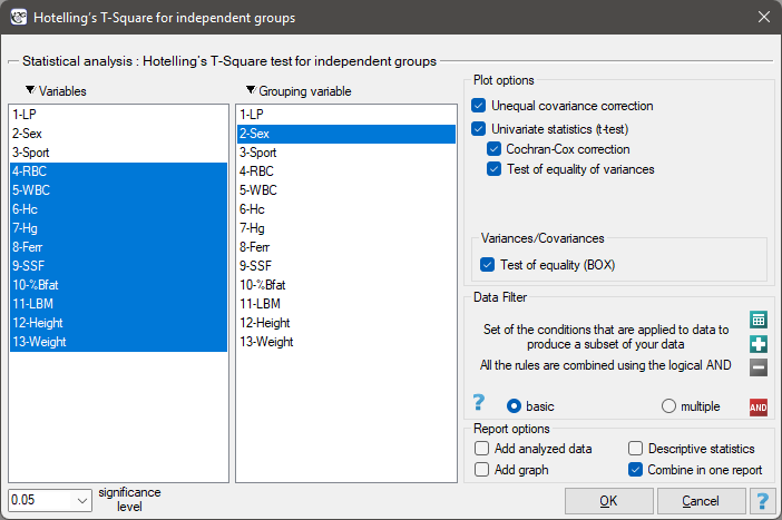
Performing and interpreting the analysis
Example 3. (sport.pqs file)
A group of athletes was studied to obtain information on health parameters such as:
| RBC – red blood cell count, | SSF – sum of skinfolds [mm], |
| WBC – white blood cell count, | % Bfat – body fat percentage, |
| Hc – haematocrit [%], | LBM – lean body mass [kg], |
| Hg – haemoglobin [g/dl], | Height [cm], |
| Ferr – ferritin [µg/l], | Body weight [kg]. |
We want to know whether women and men who practise the sports studied professionally differ in the levels of these parameters.
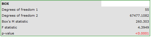
Because of differences in the covariance of the parameters analysed (Box's test \(p<0.000001\)), the analysis is performed with the correction for unequal covariance matrices enabled.
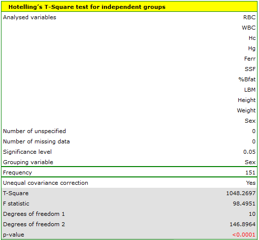
The resulting corrected Hotelling statistic is shown below.
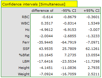
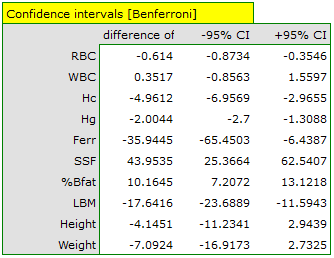
According to the simultaneous confidence intervals (and according to the intervals with the Bonferroni correction), the differences concern: RBC, Hc, Hg, ferritin, and LBM (women score lower on average), as well as SSF and % Bfat (men score lower on average). The remaining parameters – WBC, height, and body weight – do not differ significantly.
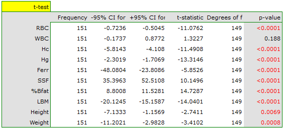
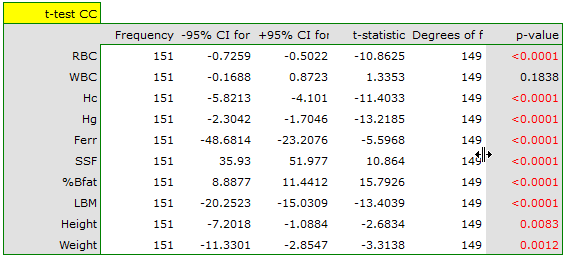
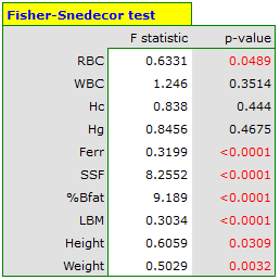
Because of its simplicity, the univariate approach – although it does not account for multiple testing or the interrelationships between variables – is the one most often used. Its results indicate that the differences concern all the parameters studied except WBC, and the results of the \(t\)-Student test are interpreted with the Cochran-Cox correction or without it, depending on whether the assumption of equal variances is met (the result of the Fisher-Snedecor test). To account for multiple testing here, one of the \(p\)-value corrections described in the Multiple comparisons section should be applied.
Hypotheses:
where:
\(\mu_x=(\mu_{x1}, \mu_{x2},..., \mu_{xk})\) – means of the variables in the first population,
\(\mu_y=(\mu_{y1}, \mu_{y2},..., \mu_{yk})\) – means of the variables in the second population.
Formulas: The test statistic is defined by:
where:
\(n=n_x+n_y-1\),
\(n_x\), \(n_y\) – the sizes of the first and second sample (the sizes of the individual variables are the same),
\(T^2 = (\overline{x}-\overline{y})^T\left(S\left(\frac{1}{n_x}+\frac{1}{n_y}\right)\right)^{-1}(\overline{x}-\overline{y})\) – the original Hotelling test statistic, which has the \(\chi^2\) distribution (recommended for samples with large sizes),
\(\overline{x}=(\overline{x}_1, \overline{x}_2,..., \overline{x}_k)\) – means of the variables in the first sample,
\(\overline{y}=(\overline{y}_1, \overline{y}_2,..., \overline{y}_k)\) – means of the variables in the second sample,
\(S\) – the pooled covariance matrix for both samples.
The test statistic has the F Snedecor distribution with \(k\) and \(n-k\) degrees of freedom.
The \(p\) value, determined on the basis of the test statistic, is compared with the significance level \(\alpha\): if \(p \le \alpha\), we reject \(\mathcal{H}_0\) in favor of \(\mathcal{H}_1\); if \(p > \alpha\), there is no reason to reject \(\mathcal{H}_0\).
Simultaneous confidence intervals
When, after performing the analysis, we look for the variables the differences concern, we calculate simultaneous confidence intervals for the mean differences:
or the intervals with the Bonferroni correction, to check whether the value 0 falls within them. If the difference can equal 0, this means the difference between the values studied may not actually exist. When using this method, keep in mind that the resulting intervals do not take into account the interrelationships between the variables (which Hotelling's test does take into account), only the effect of multiple testing.
When looking for the variables the differences concern, we can also use a univariate approach, performing separate comparisons for each variable with the \(t\)-test for independent groups. Unfortunately, this does not account for the interrelationships between variables, but the \(p\) values obtained from the \(t\)-Student test can be adjusted in the Multiple comparisons section.
Hotelling's T-square test for independent groups with correction for unequal variances
When to use this test:
This correction applies to the Hotelling's T-square test for independent groups and is calculated when the variances of the variables studied differ between the two populations.
How to set up the analysis
The correction is an option available in the same window as the Hotelling's T-square test for independent groups.
Performing and interpreting the analysis
See Example 3 above – because of the significant result of Box's test, the analysis there was in fact performed using this correction.
Formulas: The test statistic is defined by:
where:
\(n=n_x+n_y-1\),
\(n_x\), \(n_y\) – the sizes of the first and second sample (the sizes of the individual variables are equal),
\(T^2 = (\overline{x}-\overline{y})^T\left(\frac{S_x}{n_x}+\frac{S_y}{n_y}\right)^{-1}(\overline{x}-\overline{y})\) – the original Hotelling test statistic, which has the \(\chi^2\) distribution (recommended for samples with large sizes),
\(\overline{x}=(\overline{x}_1, \overline{x}_2,..., \overline{x}_k)\) – means of the variables in the first sample,
\(\overline{y}=(\overline{y}_1, \overline{y}_2,..., \overline{y}_k)\) – means of the variables in the second sample,
\(S_x\), \(S_y\) – the covariance matrices for the first and second sample.
The test statistic has the F Snedecor distribution with \(k\) and \(m\) degrees of freedom (where \(m\) is the number of degrees of freedom adjusted for the unequal variances).
The \(p\) value, determined on the basis of the test statistic, is compared with the significance level \(\alpha\): if \(p \le \alpha\), we reject \(\mathcal{H}_0\) in favor of \(\mathcal{H}_1\); if \(p > \alpha\), there is no reason to reject \(\mathcal{H}_0\).
Simultaneous confidence intervals
When, after performing the analysis, we look for the variables the differences concern, we calculate simultaneous confidence intervals for the mean differences:
or the intervals with the Bonferroni correction, to check whether the value 0 falls within them. If the difference can equal 0, this means the difference between the values studied may not actually exist. When using this method, keep in mind that the resulting intervals do not take into account the interrelationships between the variables (which Hotelling's test does take into account), only the effect of multiple testing.
When looking for the variables the differences concern, we can also use a univariate approach, performing separate comparisons for each variable with the \(t\)-test with the Cochran-Cox correction. Unfortunately, this does not account for the interrelationships between variables, but the \(p\) values obtained from the \(t\)-Student test can be adjusted in the Multiple comparisons section.
Box's test for equality of covariance matrices
When to use this test:
This test is used to compare two or more (\(m \geq 2\)) covariance matrices describing independent populations.
Assumptions
- measurement on an interval scale,
- a multivariate normal distribution in the populations studied, or normality of distribution of each variable studied in each population,
- an independent model.
How to set up the analysis
Box's test is calculated as an option in Hotelling's test for independent groups or in the MANOVA analysis.
Performing and interpreting the analysis
See Example 3.
Hypotheses:
where \(\Sigma_1, \Sigma_2, ..., \Sigma_m\) – the population covariance matrices.
Formulas: The test statistic is defined by:
where:
\(M=(n-m)\ln|S|-\sum_{j=1}^m(n_j-1)\ln|S_j|\),
\(S\) – the pooled covariance matrix,
\(S_j\) – the covariance matrix for the \(j\)-th sample,
\(b=\frac{df_1}{1-c_1-\frac{df_1}{df-2}}\),
\(df_1=\frac{k(k+1)(m-1)}{2}\),
\(df_2=\frac{df_1+2}{|c_2-c_1^2|}\),
\(k\) – the number of variables analysed,
\(n=n_1=n_2=...=n_k\) – the sample sizes of the individual variables.
The test statistic has the F Snedecor distribution with \(df_1\) and \(df_2\) degrees of freedom.
The \(p\) value, determined on the basis of the test statistic, is compared with the significance level \(\alpha\): if \(p \le \alpha\), we reject \(\mathcal{H}_0\) in favor of \(\mathcal{H}_1\); if \(p > \alpha\), there is no reason to reject \(\mathcal{H}_0\).