 PQStat
The Z test for two independent proportions
When to use this test:
The \(Z\) test for two independent proportions is used in similar situations as the \(\chi^2\) test (\(2\times2\)): when we have 2 independent samples in which the analysed feature takes one of two possible outcomes, and we want to check whether the share (proportion) of the distinguished outcome is the same in the two populations from which the samples were drawn.
Assumptions
- measurement on a nominal scale – any ordering of categories is not taken into account,
- an independent model,
- large sample size.
How to set up the analysis
Statistics \(\to\) NonParametric tests \(\to\) Z for 2 independent proportions.
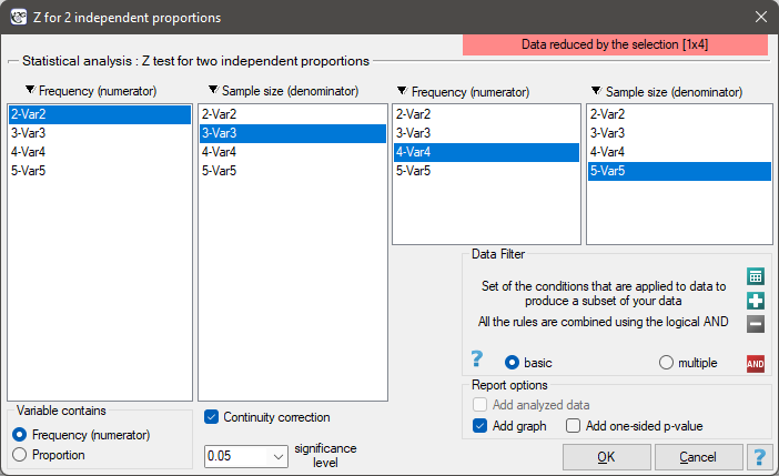
Performance and interpretation
Example 1. Example (?) cont. (sex-exam.pqs file)
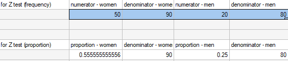
We know that \(\frac{50}{90}=55.56\%\) of all women in the sample passed the exam, and \(\frac{20}{80}=25.00\%\) of all men in the sample passed the exam. We want to check whether the pass-rate proportion differs between the sexes in the analysed population.
The data can be written in two ways – as a numerator and a denominator for each sample, or as a proportion and a denominator for each sample:
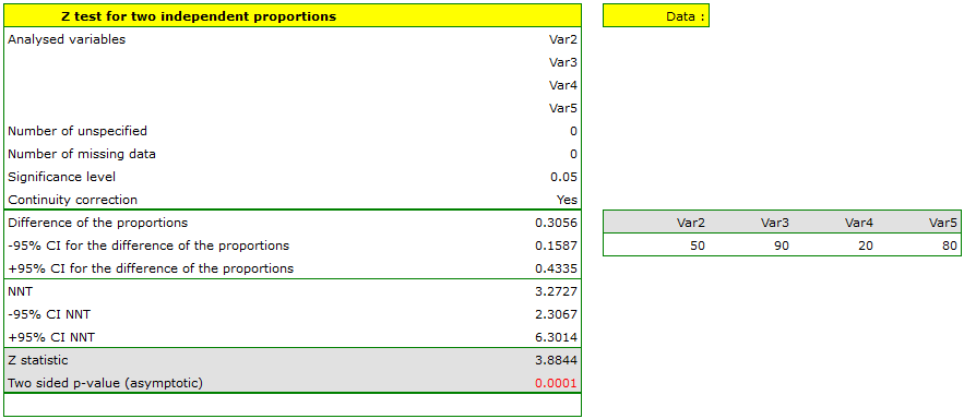
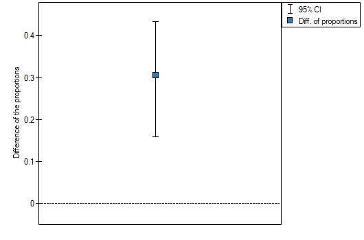
The difference between the proportions distinguished in the sample is 30.56%, and its 95% confidence interval \((15.90\%, 43.35\%)\) does not contain 0. The same conclusion is reached with the \(Z\) test with the continuity correction (\(p=0.0001\)) – similarly to the previously performed tests: the exact Fisher test, mid-p, chi-square, and chi-square with the Yates correction. The exam was passed significantly more often by women (55.56% of the sample) than by men (25.00% of the sample).
Example 2. Let us assume that a disease has a 100% mortality rate without treatment, and therapy reduces the mortality rate to 50% – this is the result of a 20-year study. We want to know how many people would need to be treated to prevent 1 death over 20 years. For this purpose, two 100-person samples were drawn from the population of diseased people: in the untreated sample all 100 patients die, in the treated sample 50 out of 100 patients survive.
| Patients – not treated | Patients – treated | ||
| sample numerator | sample size (denominator) | sample numerator | sample size (denominator) |
| 100 | 100 | 50 | 100 |
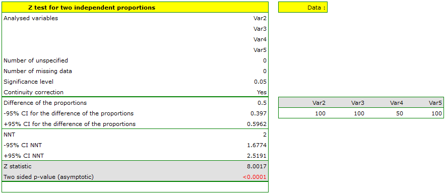
The calculated 95% confidence interval for NNT should be rounded to whole numbers, giving an NNT of 2 to 3 patients.
Example 3. A certain proportion difference in a study comparing the effectiveness of drug 1 vs drug 2 was (95%CI)\(=-0.08\) (\(-0.27\) to \(0.11\)). This negative proportion difference suggests that drug 1 was less effective than drug 2, and its use exposed patients to risk.
Definitions of measures
NNT (ang. number needed to treat) – an indicator used in medicine, denoting the number of patients who need to be treated for a specified time in order to cure one person who would not otherwise have recovered.
NNH (ang. number needed to harm) – an indicator used in medicine, denoting the number of patients whose exposure to a risk over a specified time results in harm to one person who would not otherwise have been harmed.
Definition: Let \(p_1=\frac{m_1}{n_1}\) and \(p_2=\frac{m_2}{n_2}\) denote the distinguished proportions in samples of sizes \(n_1\), \(n_2\), where \(m_1\), \(m_2\) – the frequencies of the distinguished outcome in the first and second sample.
Hypotheses:
\( \begin{array}{cl} \mathcal{H}_0: & P_1=P_2,\\ \mathcal{H}_1: & P_1\neq P_2, \end{array} \)
where \(P_1\), \(P_2\) – distinguished proportions in the first and second population.
Formulas: The test statistic is defined by:
where \(p=\frac{m_1+m_2}{n_1+n_2}\).
The test statistic modified by the continuity correction is defined by:
The statistic, with and without the continuity correction, asymptotically (for large sample sizes) has the normal distribution.
Formulas – NNT/NNH: NNT is calculated using the formula:
and is quoted when the difference \(p_1-p_2\) is positive. NNH is calculated the same way as NNT, but is quoted when the difference \(p_1-p_2\) is negative.
Interpretation: The narrower the confidence interval, the more precise the estimate. If the confidence interval for the difference in proportions contains 0 (and for NNT/NNH – contains \(\infty\)), this is an indication that the result should be treated as not statistically significant.
Confidence interval estimation method – confidence intervals for the difference between two independent proportions, from PQStat version 1.3.0, are estimated using the Newcombe-Wilson method (Bender 2001[18], Newcombe 1998[127], Wilson 1927[177]); previously the Wald method was used. The Wald method is suitable for large samples and proportion differences far from 0 or 1 – for small samples and values close to these extremes it can lead to unreliable results (Newcombe 1998[127], Miettinen 1985[124], Beal 1987[17], Wallenstein 1997[169]). The Newcombe-Wilson method is also suitable for extreme values of proportions.