 PQStat
The \(t\)-test for independent groups
When to use this test:
The \(t\)-test for independent groups is used to verify the hypothesis about the equality of means of an analysed variable in two populations – e.g. when comparing the value of some feature between two independent, unrelated groups (women and men, a treated group and a control group).
Assumptions
- measurement on an interval scale,
- normality of distribution of the analysed variable in both populations,
- an independent model,
You do not need to check the equality of variances in both groups yourself – PQStat does this automatically and selects the appropriate version of the test (see How to set up the analysis).
The \(t\)-test with the Cochran-Cox adjustment
The Cochran-Cox adjustment (1957)[44] is a variant of the \(t\)-test for independent groups, applied automatically when the variances of the analysed variable in the two populations differ significantly. The assumptions and purpose of the test are the same as for the basic variant – only the way the test statistic and the degrees of freedom are calculated is different (see For those interested).
How to set up the analysis
Statistics \(\to\) Parametric tests \(\to\) \(t\)-test for independent groups (or via the Wizard).
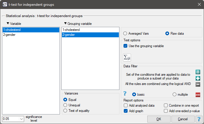
In the option concerning variances, choose one of the settings:
- equal – the \(t\)-test for independent groups will be calculated,
- different – the \(t\)-test with the Cochran-Cox adjustment will be calculated,
- check equality – the program will calculate the Fisher-Snedecor test itself and, on this basis, automatically select the appropriate variant of the test.
Performing and interpreting the analysis
Example 1. (cholesterol.pqs file)
Five hundred subjects each were drawn from a population of women and a population of men living in Poland, over 40 years of age. The study concerned the assessment of cardiovascular disease risk. Among the parameters studied is the total cholesterol concentration. The purpose of this study is to compare men and women with respect to this value – we want to show that these populations already differ at the level of total cholesterol concentration, and not only in the individual cholesterol fractions.
The distribution of age in both groups is a normal distribution (this was checked with the Lilliefors test). The mean total cholesterol concentration in the male group was \(\overline{x}_1=201.1\), and the standard deviation \(sd_1=47.6\); in the female group \(\overline{x}_2=191.5\) and \(sd_2=43.5\), respectively. The Fisher-Snedecor test indicates small, but statistically significant (\(p=0.0434\)), differences in variances. The Student's \(t\)-test with the Cochran-Cox adjustment will be used in the analysis.
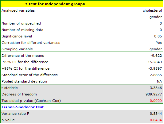
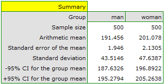
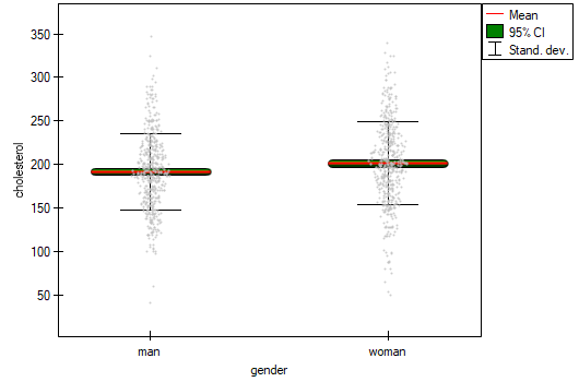
The \(p\) value, calculated on the basis of the test statistic, is always compared with the assumed significance level \(\alpha\): if \(p \le \alpha\), the difference between the means is statistically significant; if \(p > \alpha\), there are no grounds to claim that the groups differ. It is also worth reporting the effect size (Cohen's d) – statistical significance alone does not indicate how large the difference is; with large samples, even small differences can turn out to be statistically significant.
Definitions of measures
Cohen's d – a standardized effect-size measure that determines how large a part of the observed variation in the data is the observed difference between the means. Unlike the \(p\) value, it does not depend on sample size, which makes it possible to assess the practical significance of a difference, not just its statistical significance.
The \(t\)-test for independent groups
Hypotheses:
\(\begin{array}{cc} \mathcal{H}_0: & \mu_1=\mu_2,\\ \mathcal{H}_1: & \mu_1\ne\mu_2. \end{array}\)
where \(\mu_1\), \(\mu_2\) – means of the analysed variable in the first and the second population.
Formulas:
The test statistic is defined by:
where \(\overline{x}_1, \overline{x}_2\) – means of the 1st and the 2nd sample, \(n_1, n_2\) – the 1st and the 2nd sample size, \(sd_1^2, sd_2^2\) – variances of the 1st and the 2nd sample. The test statistic has the \(t\)-Student distribution with \(df=n_1+n_2-2\) degrees of freedom.
Pooled standard deviation:
Standard error of the difference of means:
Cohen's d formula:
Cohen's d is calculated using the formula:
When interpreting an effect, researchers often use general guidelines proposed by Cohen [47], defining a small (0.2), medium (0.5) and large (0.8) effect size.
The \(t\)-test with the Cochran-Cox adjustment
Formulas:
The test statistic is defined by:
The test statistic has the \(t\)-Student distribution with the degrees of freedom proposed by Satterthwaite (1946)[148] and calculated using the formula: