One-way MANOVA for independent groups

When to use this test:

One-way MANOVA (multivariate analysis of variance) is an extension of the one-way ANOVA for independent groups. It lets you check the equality of the means of \(k\) variables studied across several (\(m\geq2\)) populations. Unlike using ANOVA repeatedly (separately for each variable), MANOVA examines the differences between populations simultaneously for multiple variables, while taking their mutual correlation into account. This approach is also used as an alternative to the ANOVA for dependent groups, since it does not require the sphericity assumption to be met. We recommend reading about Hotelling's T-square beforehand.

Assumptions

measurement on an interval scale,
a multivariate normal distribution in each population, or normality of distribution of each variable studied in each population,
an independent model,
equality of the covariance matrices, or equality of variances of the variables studied for the populations compared – a condition that is especially important for groups of different sizes.

Note! The principle behind MANOVA (as with Hotelling's tests) is identical to constructing multivariate confidence-interval ellipses around the centres determined by the means (see the example interpreting the Hotelling test ellipse for a single sample). Because of this, a univariate analysis (which does not take the interrelationships between the variables into account) will often fail to give an identical result.

How to set up the analysis

Statistics \(\to\) Parametric tests \(\to\) One-way MANOVA for independent groups.

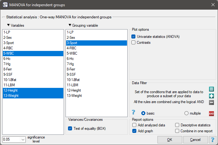
Performing and interpreting the analysis

Example 1. (sport.pqs file)

A group of athletes was studied to obtain information on health parameters, among others such as:
WBC – white blood cell count,
Height [cm],
Body weight [kg].
We want to know:

whether athletes who professionally practise three types of sport – “team sports”(such as basketball, volleyball, etc.), “track”(such as 100m, 400m, etc.), and “water sports”(such as swimming, rowing, etc.) – differ in the levels of these parameters;
whether athletes practising sports that require great effort, such as “track”and “water sports”, differ in the levels of these parameters from those practising “team sports”.

Re. 1)
Hypotheses:

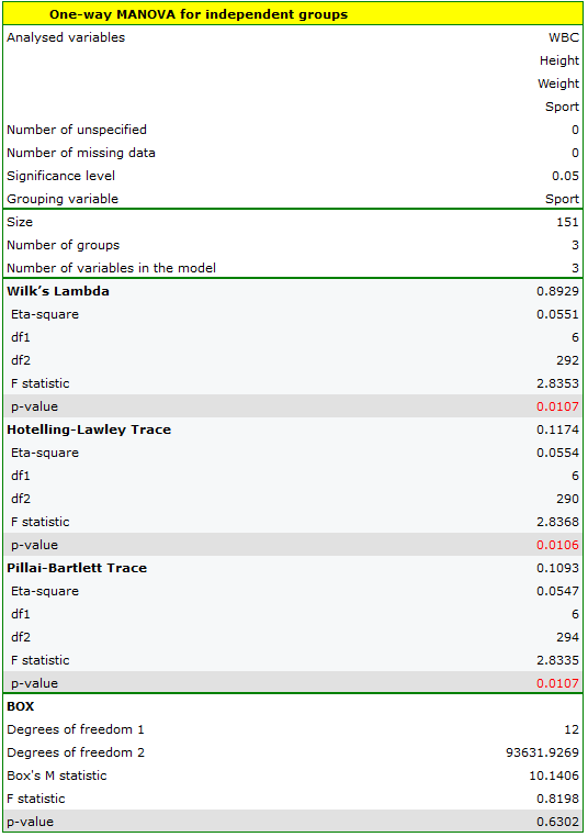
\[ \begin{array}{cl} \mathcal{H}_0: & \text{the means of the parameters analysed are the same}\\ & \text{for athletes practising the individual types of sport,}\\ \mathcal{H}_1: & \text{at least one parameter has a different mean value}\\ & \text{for the populations compared.}\\ \end{array} \]

The result of Box's test (\(p=0.63025\)) allows a MANOVA-type analysis to be calculated.

significant Wilks' Lambda, Hotelling-Lawley trace, and Pillai-Bartlett trace (statistically significant, \(\alpha=0.05\))

The populations of athletes studied differ with regard to the parameters analysed.

To determine which variables the differences concern, we perform a univariate ANOVA analysis.

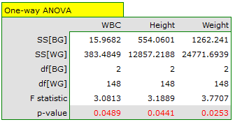
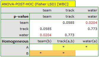
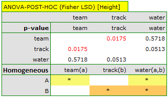
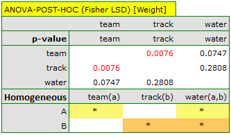
The results obtained should be treated with caution. Although they indicate significant differences in all the parameters compared, the \(p\) values returned are close to the boundary of statistical significance (for WBC \(p=0.04885\), for height \(p=0.04406\), for weight \(p=0.02528\)). In addition, when interpreting them, keep in mind that they take into account neither the mutual correlation of the parameters nor multiple testing. Accounting for multiple testing here would require applying one of the \(p\)-value corrections described in the Multiple comparisons section.

Re. 2)
Hypotheses:

\[ \begin{array}{cl} \mathcal{H}_0: & \text{the means of the parameters analysed for }\text{team sports}\\ & \text{do not differ from the corresponding means of athletes from the other two groups,}\\ \mathcal{H}_1: & \text{at least one parameter has a different mean value}\\ & \text{for the populations compared.}\\ \end{array} \]

To check whether the above hypotheses hold, we set an appropriate contrast in the analysis window. We enter 2 as the contrast value for team sports, and \(-1\) for track and for the disciplines defined as water sports.

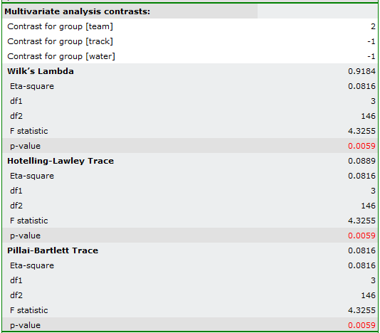
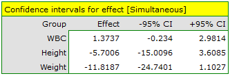
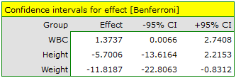
\(p=0.00592\) for Wilks' Lambda, the Hotelling-Lawley trace, and the Pillai-Bartlett trace (statistically significant, \(\alpha=0.05\))

Athletes practising sports that require great effort differ in the parameters analysed from those practising team sports.

We do not observe these differences in the simultaneous intervals, but on the basis of the Bonferroni intervals we can conclude that the difference concerns weight and WBC. WBC values are higher in the team-sports group, and body weight is significantly lower in this group.

Definitions of measures

Partial \(\eta^2\) – a measure of effect size expressing the proportion of explained variance to total variance associated with a given factor. In the one-way MANOVA model for independent groups, it indicates what proportion of the within-subject variability in outcomes can be attributed to the factor under study that defines the independent groups.

Contrasts (univariate analysis) – when the analysis performed aims to compare selected populations or a selected pattern of populations, we perform a contrast analysis, analogous to contrasts in univariate analysis, but taking into account the interrelationships between the variables.

FOR THOSE INTERESTED

Hypotheses:

\[\begin{array}{cl} \mathcal{H}_0: & \mu_1=\mu_2=...=\mu_m,\\ \mathcal{H}_1: & \text{not all }\mu_i\text{ are equal,} \end{array}\]

where:
\(\mu_i=(\mu_{i1}, \mu_{i2},..., \mu_{ik})\) – means of the variables in the \(i\)-th population,
\((i=1,2,...,m)\),
\((j=1,2,...,k)\).

Explanation:
Several coefficients are used in MANOVA analyses. The best known is Wilks' Lambda. The Pillai-Bartlett trace is the most conservative, but relatively robust to violations of the MANOVA assumptions, and is preferred for small samples. The Hotelling-Lawley trace, in turn, is the least conservative of the three tests proposed. Pioneering work on the development of these techniques was begun by Wilks (1932)[178], Pillai (1955)[136], Lawley (1938)[101], Hotelling (1951)[87], and Roy (1939)[144].

The test statistics are based on matrices of sums of squares and cross products (\(SSCP\)). The total matrix \(T=SSCP\) is split into two matrices: the first is associated with the hypothesis analysed and is denoted by \(H\) (the between-groups sum-of-squares and cross-products matrix), and the second concerns the residuals (errors) and is denoted by \(E\) (the within-groups sum-of-squares and cross-products matrix).

Wilks' Lambda – formulas:
The value of Lambda is defined as follows:

\[ \Lambda=\frac{|E|}{|H+E|} \]

The test statistic is defined by:

\[ F=\frac{1-\Lambda^{\frac{1}{b}}}{\Lambda^{\frac{1}{b}}}\frac{df_2}{df_1} \]

where \(df_1=k(m-1)\), \(df_2=ab-c\), and \(a\), \(b\), \(c\) are coefficients that depend on the number of variables analysed and the number of populations compared.

The Hotelling-Lawley trace – formulas:
The Hotelling-Lawley trace is defined as follows:

\[ T_0=trace(HE^{-1}) \]

The test statistic is defined by:

\[ F=\frac{T_0^2}{s}\frac{df_2}{df_1} \]

where \(df_1=s(2t+s+1)\), \(df_2=2(su+1)\), and \(s\), \(t\), \(u\) are coefficients that depend on the number of variables analysed and the number of populations compared.

The Pillai-Bartlett trace – formulas:
The Pillai-Bartlett trace is defined as follows:

\[ V=trace(H(H+E)^{-1}) \]

The test statistic is defined by:

\[ F=\frac{V}{s-V}\frac{df_2}{df_1} \]

where \(df_1=s(2t+s+1)\), \(df_2=s(2u+s+1)\), and \(s\), \(t\), \(u\) are coefficients that depend on the number of variables analysed and the number of populations compared.

Each of the above test statistics has the F Snedecor distribution with \(df_1\) and \(df_2\) degrees of freedom.

The \(p\) value, determined on the basis of the test statistic, is compared with the significance level \(\alpha\): if \(p \le \alpha\), we reject \(\mathcal{H}_0\) in favor of \(\mathcal{H}_1\); if \(p > \alpha\), there is no reason to reject \(\mathcal{H}_0\).

Partial \(\eta^2\) – formula:

\[ \eta^2=\frac{F\cdot df_1}{F\cdot df_1+df_2} \]

Contrasts (univariate analysis)
For effect sizes, simultaneous confidence intervals or confidence intervals with the Bonferroni correction can also be calculated. When using these intervals, however, keep in mind that they do not take into account the interrelationships between the individual variables (which MANOVA does take into account), only the effect of multiple testing.

When looking for the variables the differences concern, we can also use a univariate approach, performing separate comparisons for each variable with the ANOVA for independent groups. Unfortunately, this does not account for the interrelationships between variables, but the \(p\) values obtained from ANOVA can be adjusted in the Multiple comparisons section.