CLUSTER ANALYSIS

Cluster analysis is the search, within the data, for groups of similar objects (e.g. customers, patients, species) – such that the objects inside one group (a cluster) are as similar to one another as possible, while objects from different clusters differ as much as possible. Two main families of methods are distinguished: hierarchical methods, which build an entire hierarchy of possible partitions, and non-hierarchical methods, of which the most popular is the k-means method. Both families of methods base their operation on a similarity matrix, i.e. on information about how similar (or how different) the individual objects are.
In exactly the same way that objects (e.g. studied subjects) are grouped, variables (features) can also be grouped – e.g. in order to identify variables carrying similar information. In this chapter, the grouping methods will be described using the grouping of objects as an example.

Hierarchical methods

When to use:

Hierarchical cluster analysis is used when we want to see not just a single, final division of the objects into groups, but the entire hierarchy of possible divisions – from single objects, through progressively larger clusters, up to a single cluster containing all the objects. The method builds this hierarchy step by step, joining at each step the two most similar (nearest) objects or clusters, on the basis of the similarity matrix. This lets the researcher later decide for themselves at what level to "cut" the resulting hierarchy in order to obtain the number of clusters they are interested in.

Assumptions

the possibility of calculating the distance/similarity between objects – the choice of an appropriate measure depends on the measurement scale of the analysed variables (see Similarity matrix),
standardisation of the variables before calculating the similarity matrix, so that none of them (e.g. one expressed by much larger numbers) dominates the others when building the clusters,
the absence of grossly atypical (outlying) observations, which could significantly distort the distances between the remaining objects.

Note! To ensure a balanced influence of all variables on the elements of the similarity matrix, the data should be standardised by selecting the appropriate option in the analysis window. Without standardisation, variables expressed by larger numbers have a greater influence on the result obtained.

Definitions of measures

Similarity of objects

In the course of work related to cluster analysis, similarity or distance measures play a fundamental role. The mutual similarity of the objects is placed in the similarity matrix. The large variety of methods for determining the distance/dissimilarity between objects allows the choice of measures that best reflect the actual relations. Distance and similarity measures are described in more detail in the Similarity matrix section.
Cluster analysis bases its operation on searching for clusters inside the similarity matrix. Such a matrix is built during the course of performing the cluster analysis. For the cluster analysis to produce the desired results, when choosing the way of calculating the distance it should be remembered that larger numerical values in the similarity matrix should indicate greater dissimilarity of the objects, and smaller values their similarity.

Note! To increase the influence of the selected variables on the elements of the similarity matrix, appropriate weights should be indicated when setting up the way of defining the distance, while at the same time remembering to standardise the data.

For example, for people wanting to take care of a dog, grouping dogs according to size, coat colour, tail length, character, breed, etc. will make the choice easier. However, treating all characteristics identically may result in completely dissimilar dogs being placed in one group. For most of us, on the other hand, a dog's size and character matter more than its tail length, so when grouping, the similarity measures should be set so that it is precisely size and character that carry the greatest weight in building the clusters.

Methods of linking objects and clusters

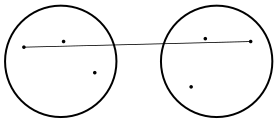
Single linkage method (nearest neighbour) – the distance between clusters is determined by the distance between the objects of each cluster that lie closest to each other.
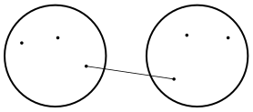
Complete linkage method (farthest neighbour) – the distance between clusters is determined by the distance between the objects of each cluster that lie farthest from each other.
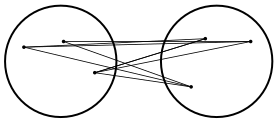
Average linkage method – the distance between clusters is determined by the average distance between all pairs of objects located within two different clusters.
Weighted average linkage method – analogously to the average linkage method, this involves calculating the average distance, but this average is weighted by the number of elements in each cluster. As a result, this method should be chosen when we expect to obtain clusters of similar sizes.
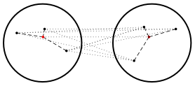
Ward's method – based on the principle of analysis of variance – it calculates the difference between the sums of squared deviations of the distances of the individual objects from the centroid of the clusters to which those objects belong. This method is chosen most often because of its fairly universal character.

Dendrogram
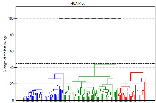
The result of a cluster analysis carried out by a hierarchical method is presented by means of a dendrogram. A dendrogram is a tree-like form showing the relationships between the individual objects, obtained from the analysis of the similarity matrix. The cutoff level of the dendrogram determines the number of clusters into which we want to divide the collected objects. We define the way the cutoff is made by specifying, as a percentage, the length of the linkage at which the cut will occur, where 100% is the length of the last, and at the same time the longest, linkage in the dendrogram.

How to set up the analysis

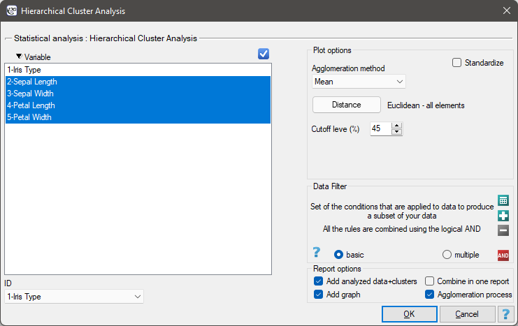
The window with the hierarchical cluster analysis options is opened through the Advanced statistics\(\to\)Grouping and reduction\(\to\)Hierarchical cluster analysis menu.

Performing and interpreting the analysis

Example (1) cont. (iris.pqs file)
The analysis will be performed on the classic data set concerning the division of iris flowers into 3 varieties, on the basis of the width and length of the petals and sepals (R.A. Fisher, 1936[60]). Because this data set contains information about the actual variety of each flower, once the cluster analysis has been performed, it is possible to determine the accuracy of the division made.
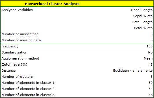
We assign the flowers to particular groups on the basis of columns 2 to 5. We choose the way of calculating the distance, e.g. the Euclidean distance, and the linkage method, e.g. the average. Specifying the cluster cutoff level will let us cut the dendrogram in such a way that clusters are formed – in the case of this analysis we want to obtain 3 clusters, and to achieve this we change the cutoff level to 45%. We also attach data+clusters to the report.

The dendrogram chart shows the order of the linkages and their length.

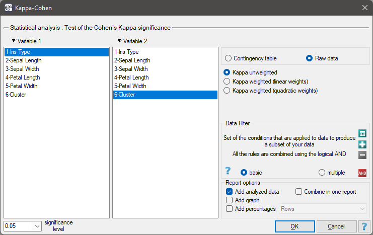
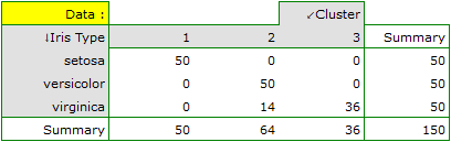
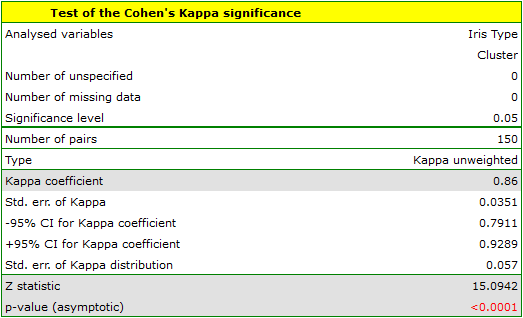
To examine whether the extracted clusters represent the 3 actual iris varieties, we can copy the column containing the information on cluster membership from the report and paste it into the datasheet. Like the clusters, the varieties are also described numerically through Codes/Labels/Format, so an agreement analysis can easily be carried out. We will check the agreement of our results with the actual membership of a given flower in the corresponding species using the Cohen's Kappa method.

For the example presented, the observed agreement is shown by the table:

Cohen's Kappa \(=0.86\) (statistically significant)

The virginica variety can be confused with versicolor, which is why we observe 14 misclassifications here. The Kappa agreement coefficient itself is, however, statistically significant and equals 0.86, which shows a high level of agreement between the obtained clusters and the actual flower variety.

The k-means method

When to use:

The k-means method is used when it is already known (or assumed) in advance into how many groups (\(k\)) we want to divide the objects, and we are primarily interested in a single, final division – without building an entire hierarchy, as in the hierarchical methods. The method is modelled on the algorithm initially proposed by Stuart Lloyd and published in 1982[109]. Objects are moved between clusters so that the dissimilarity of the objects inside each cluster is as small as possible, and the distances between clusters as large as possible.

Assumptions

measurement of the variables allowing the Euclidean distance between objects to be calculated (the algorithm is based on the matrix of Euclidean distances),
a number \(k\) of sought clusters assumed in advance,
standardisation of the variables, so that none of them dominates the others when building the clusters (analogously to the hierarchical methods).

Definitions of measures

In this method, the objects are divided into a predetermined number of \(k\) clusters. The initial clusters are improved in the course of the agglomeration procedure, by moving objects between them so that the dissimilarity of the objects within a cluster is as small as possible, and the distances between clusters as large as possible. The algorithm operates on the basis of the matrix of Euclidean distances between objects, and the parameters needed in the agglomeration procedure of the k-means method are: the starting centres and the stopping criterion. The starting centres are the objects from which the algorithm will begin building the clusters, and the stopping criterion defines how the algorithm is to be stopped.
Starting centres
The choice of starting centres has a fundamental effect on the convergence of the k-means algorithm towards obtaining suitable clusters. The starting centres can be selected in two ways:

k-means++ – the optimal selection of starting points, using the k-means++ algorithm proposed in 2007 by David Arthur and Sergei Vassilvitskii[1]. It guarantees that the optimal solution of the k-means algorithm is obtained with as few iterations as possible. The algorithm uses an element of randomness, so the results obtained may differ slightly between successive runs of the analysis. If the data do not form natural clusters, using k-means++ will give quite different results in successive runs of the k-means analysis. High reproducibility of the results, on the other hand, indicates the possibility of achieving a good division into separate clusters.
First n – lets the user indicate the points that are to be the starting centres, by placing these objects in the first positions in the data table.

The stopping criterion is the moment at which the membership of the points in the classes no longer changes, or the number of repetitions of the steps of the agglomeration procedure reaches the number of iterations set by the user.
Given the way the k-means cluster analysis algorithm works, a natural consequence of it is to compare the resulting clusters by means of a one-way analysis of variance (ANOVA) for independent groups.

How to set up the analysis

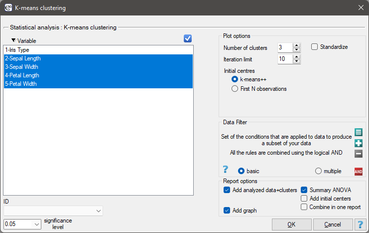
The window with the k-means cluster analysis options is opened through the Advanced statistics\(\to\)Grouping and reduction\(\to\)K-means cluster analysis menu.

Performing and interpreting the analysis

Example (1) cont. (iris.pqs file)
The analysis will be performed on the classic data set concerning the division of iris flowers into 3 varieties, on the basis of the width and length of the petals and sepals (R.A. Fisher, 1936[60]).
We assign the flowers to particular groups on the basis of columns 2 to 5. We also indicate that we want to divide the studied flowers into 3 groups.

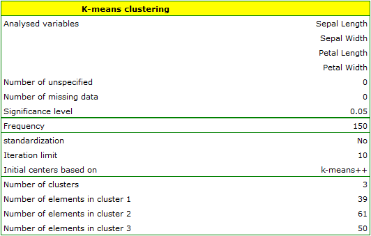
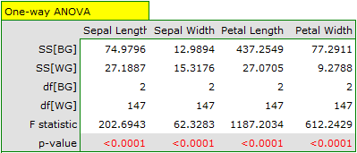
ANOVA result statistically significant for each of the 4 dimensions

As a result of the analysis performed, 3 clusters were formed, which differ statistically significantly in every studied dimension, i.e. for petal width, petal length, sepal width, and sepal length.

The difference can be observed on the charts, where, for two selected dimensions, we show the membership of the individual points in a cluster:

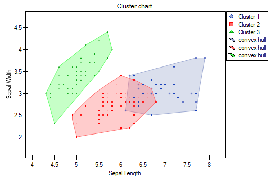
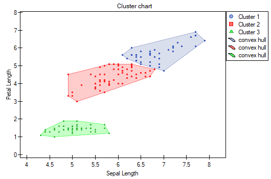
Repeating the analysis may give slightly different results, but the variability obtained will not be large. This shows that the data submitted to the analysis do form natural clusters, and that carrying out a cluster analysis is justified in this case.

Note! After running the analysis a few times, we can select the result that interests us most, and then set the data that form the starting centres at the beginning of the sheet – the analysis carried out on the basis of starting centres chosen as First N observations will then consistently produce the result we selected.

Note! To find out whether the clusters represent the 3 actual iris varieties, we can copy the information on cluster membership from the report and paste it into the datasheet. The agreement of our results with the actual membership of a given flower in the corresponding species can be checked analogously as for the hierarchical cluster analysis.

FOR THOSE INTERESTED

Agglomeration procedure – hierarchical methods

Following the indicated linkage method, the algorithm finds a pair of similar objects in the similarity matrix and joins them into a cluster;
The dimension of the similarity matrix is reduced by one (two objects are replaced by one), and the distances in the matrix are recalculated;
Steps 2-3 are repeated until a single cluster containing all objects is obtained.

Agglomeration procedure – the k-means method

Selection of the starting centres;
On the basis of the similarity matrix, the algorithm assigns each object to the nearest centre;
Corrected centres are determined for the resulting clusters;
Steps 2-3 are repeated until the stopping criterion is met.