The Mann-Whitney U test

When to use this test:

The Mann-Whitney \(U\) test is used when comparing two independent groups on the same characteristic, and the data do not meet the assumptions of the \(t\)-test for independent groups (e.g. they are not normally distributed). It checks whether the results in the two groups differ (assuming that the distributions of the variable in both groups are fairly similar – the comparison of rank variances can be checked with the Conover rank test).

The test is also known as the Wilcoxon Mann-Whitney test (Mann and Whitney (1947)[113] and Wilcoxon (1949)[176]).

Assumptions

measurement on an ordinal scale or an interval scale,
an independent model.

How to set up the analysis

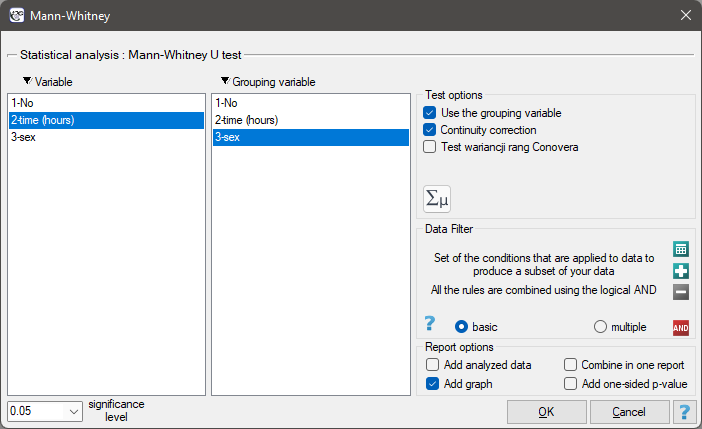
Statistics \(\to\) NonParametric tests \(\to\) Mann-Whitney (or via the Wizard).

Step 1. Indicate the grouping variable (e.g. sex) and the outcome variable (e.g. time spent in front of the computer).

Step 2. Run the analysis.

Performance and interpretation

Example 1. (computer.pqs file)
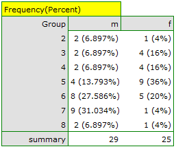
It was hypothesised that at a certain university, male math students spend statistically more time in front of a computer screen than female math students. To verify this, a sample of 54 people (25 women and 29 men) was drawn from the population of people studying math at this university. These people were asked how many hours a day they spend in front of the computer screen. The following results were obtained: (time, sex): (2, k) (2, m) (2, m) (3, k) (3, k) (3, k) (3, k) (3, m) (3, m) (4, k) (4, k) (4, k) (4, k) (4, m) (4, m) (5, k) (5, k) (5, k) (5, k) (5, k) (5, k) (5, k) (5, k) (5, k) (5, m) (5, m) (5, m) (5, m) (6, k) (6, k) (6, k) (6, k) (6, k) (6, m) (6, m) (6, m) (6, m) (6, m) (6, m) (6, m) (6, m) (7, k) (7, m) (7, m) (7, m) (7, m) (7, m) (7, m) (7, m) (7, m) (7, m) (8, k) (8, m) (8, m).

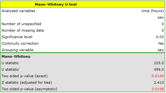
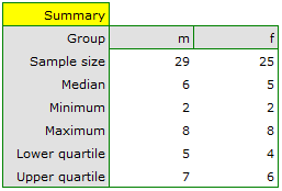
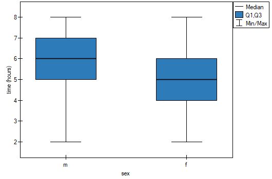
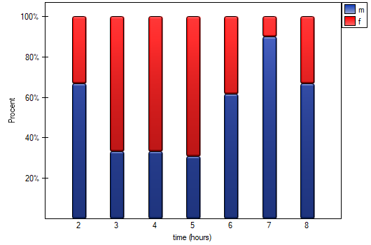
\(p=0.0149\) (exact \(U\) statistic, statistically significant, \(\alpha=0.05\))

There are statistically significant differences between female and male math students in the amount of time spent in front of the computer – female students spend less time in front of the computer than male students.

The \(p\) value, calculated on the basis of the test statistic, is always compared with the assumed significance level \(\alpha\): when \(p \le \alpha\), the difference is statistically significant; when \(p > \alpha\), there is no reason to claim that the groups differ. The same decision would be reached on the basis of the \(Z\) statistic without the continuity correction (\(p=0.0154\)) and with it (\(p=0.0158\)). The difference can be described using the median, quartiles, and the largest and smallest values, seen in a box-and-whisker plot, or using a table of counts and percentages (run in the analysis window by setting descriptive statistics ) or a column plot. It is also worth reporting the effect size (Cohen's d) – statistical significance alone does not indicate how large the difference is.

Definitions of measures

r (effect size) – a measure of effect strength based on a transformation of the test statistic \(Z\); it ranges from 0 (no effect) to 1 (maximum effect).

Cohen's d – a standardized effect-size measure, calculated here from \(r\) following the standard conversion used in meta-analyses. It makes it possible to assess the practical significance of a difference regardless of sample size.

FOR THOSE INTERESTED

Hypotheses:
Hypotheses concern the equality of mean ranks for the compared populations, or are simplified to medians:

\(\begin{array}{cl} \mathcal{H}_0: & \phi_1=\phi_2,\\ \mathcal{H}_1: & \phi_1\neq\phi_2, \end{array}\)

where \(\phi_1, \phi_2\) – distributions of an analysed variable in the 1st and the 2nd population.

Formulas:
Depending on the sample size, the test statistic is calculated using different formulas. For a small sample size:

\[ U=n_1n_2+\frac{n_1(n_1+1)}{2}-R_1, \]

\[ U'=n_1n_2+\frac{n_2(n_2+1)}{2}-R_2, \]

where \(n_1, n_2\) are sample sizes, \(R_1, R_2\) are rank sums for the samples. Standardly, the smaller of \(U\) or \(U'\) is interpreted. This statistic has the Mann-Whitney distribution and does not contain any correction for ties. The value of the exact probability of the Mann-Whitney distribution is calculated with the accuracy up to the hundredth place of the fraction. For a large sample size:

\[ Z=\frac{U-\frac{n_1n_2}{2}}{\sqrt{\frac{n_1n_2(n1+n_2+1)}{12}-\frac{n_1n_2\sum (t^3-t)}{12(n_1+n_2)(n_1+n_2-1)}}}, \]

where \(U\) can be replaced with \(U'\), \(t\) – number of cases included in a tie. The formula for the \(Z\) statistic includes the correction for ties, used when ties occur (if there are none, the correction is not calculated, since \(\frac{n_1n_2\sum (t^3-t)}{12(n_1+n_2)(n_1+n_2-1)}=0\)). The \(Z\) statistic asymptotically (for large sample sizes) has the normal distribution. The Mann-Whitney test with the continuity correction (Marascuilo and McSweeney (1977)[117]) – used to guarantee that the test statistic can take all real-number values, in line with the normal-distribution assumption:

\[ Z=\frac{\left|U-\frac{n_1n_2}{2}\right|-0.5}{\sqrt{\frac{n_1n_2(n1+n_2+1)}{12}-\frac{n_1n_2\sum (t^3-t)}{12(n_1+n_2)(n_1+n_2-1)}}}. \]

Formulas (effect size measures):
\(r\) is calculated using the formula \(r=\left|Z/(n_1+n_2)\right|\) [68], and Cohen's d:

\[ d=\frac{2r}{\sqrt{1-r^2}} \]

When interpreting an effect, researchers often use general guidelines proposed by Cohen [47] defining small (0.2), medium (0.5) and large (0.8) effect sizes.