Comparing multiple regression models

When to use:

Multiple linear regression provides the ability to analyse many independent variables simultaneously. This raises the problem of choosing the optimal model. In the flood of information carried by a model that is too large, important information can be lost. A model that is too small may omit those features that could reliably describe the phenomenon studied – it is not the number of variables in the model but their quality that determines the quality of the model. Selecting independent variables requires knowledge and experience related to the phenomenon studied. It should be remembered that the model should contain variables strongly correlated with the dependent variable and weakly correlated with each other.

Definitions of measures

There is no single simple statistical rule that determines the number of variables needed in a model. We most often use measures of model fit for comparison, such as: \(R_{adj}^2\) – the adjusted value of the multiple coefficient of determination (the higher the value, the better the model fit), \(SE_e\) – the standard error of estimation (the lower the value, the better the model fit), or the information criteria AIC, AICc, BIC (the lower the value, the better the model). For this purpose, the F-test based on the multiple coefficient of determination \(R^2\) can also be used, which is used to verify the hypothesis that the fit of both compared models is equally good.

If the compared models do not differ significantly, we should select the one with fewer variables – a lack of difference means that the variables present in the full model but absent from the reduced model do not carry significant information. If, on the other hand, the difference in model fit quality is statistically significant, this means that one of them (the one with more variables, a higher \(R^2\), or a lower information criterion value) is significantly better than the other.

Manual comparison of models consists in building 2 models:

the full model – the model with more variables,
the reduced model – the model with fewer variables; such a model is created from the full model by removing variables that are unnecessary from the point of view of the phenomenon studied.

The choice of independent variables in the compared models, and then the choice of the better model based on the comparison results, belongs to the researcher.

Automatic model selection – the program builds successive models itself and indicates the best one according to the chosen criterion.

Model terms. The unit that the automatic methods add to or remove from the model is a term: a single variable, a whole dummy variable (all its 0–1 columns at once) or an interaction. The hierarchy principle applies: an interaction can be in the model only when its main effects are in it, and only the interaction can be removed before them.

The selection criterion is chosen in the analysis window:

AIC, AICc or BIC – information criteria; the model with the lower value of the criterion is better. A move (adding or removing a term) is accepted only when it lowers the criterion;
\(p\) of the nested test – the F-test comparing the model before and after the change, with a given \(p\) threshold. A term is removed when \(p\) is greater than the threshold, and added when \(p\) is smaller than the threshold. The same \(p\) value is shown in the report as the comparison of neighbouring models;
validation error – the prediction error (RMSE) determined on observations that did not take part in fitting the model (described below: Out-of-sample evaluation of models). A move is accepted only when it reduces this error. The criterion requires the Validation option to be switched on – choosing it while validation is off switches cross-validation on.

Selection methods:

backward elimination – starts from the model with all the variables; in each step the term whose removal lowers the criterion the most is removed; it ends when no removal lowers the criterion any further;
forward selection – starts from the null model (intercept only); in each step the term that lowers the criterion the most is added; it ends when no addition lowers the criterion any further;
bidirectional stepwise – starts from the null model; in each step both additions and removals of terms are considered and the best move is chosen; it ends when no move improves the criterion;
all subsets – all models consistent with the hierarchy principle are fitted (a maximum of 15 terms), and the best model of each size is presented in the report; this method uses the information criteria or the validation error (the \(p\) criterion is not available in it).

All the models are computed on the same set of observations – rows with missing values in any of the candidate variables are discarded once, before the analysis. Thanks to this, the information criteria and the comparison tests are comparable between models.

The report contains: the selection method and criterion, the number of terms and of fitted models, the information criteria of the null model, the successive models of the selection path (each with the fit measures \(R_{adj}^2\), \(SE_e\), AIC, AICc, BIC and the table of coefficients) and the comparison of each neighbouring pair of models with the F-test (the statistic, degrees of freedom, \(p\) value). The best model according to the chosen criterion is marked in the report. If no term improves the null model, the report states that the null model is the best. With the all subsets method, neighbouring models may not be nested – in that case the F-test is not performed.

Note! The \(p\) values and confidence intervals in an automatically selected model are too optimistic, because the same data set was used both to select the variables and to estimate their effects. Automatic selection should be treated as an aid in searching for a model, and the final choice should be based on subject-matter knowledge. The selected model should be built again in the Multiple regression window and its assumptions verified.

Out-of-sample evaluation of models

The fit measures (\(R_{adj}^2\), \(SE_e\)), the information criteria and the tests are determined on the same observations on which the coefficients of the model were estimated. Such an assessment is too optimistic: the model also adapts to the accidental features of the sample, so it usually predicts new observations worse than its fit would suggest, and the more variables in the model, the larger this difference. Selection based only on the training set therefore does not always indicate the model that will perform best on new data. For this reason, the analysis window makes it possible to evaluate the models on observations that did not take part in fitting them (the Validation option):

\(k\)-fold cross-validation – the observations are randomly divided into \(k\) parts (folds) of similar size. Each model is fitted \(k\) times, each time leaving one part out, and is used to predict the values of the dependent variable in the part left out. Each observation is thus predicted exactly once – by a model that „has not seen” it. The models presented in the report (coefficients, fit measures, information criteria, tests) are fitted on all the observations, and the validation measures supplement them. The most common choices are \(k=5\) or \(k=10\);
random test set – a given percentage of the observations is randomly set aside as the test set. All the models are fitted only on the remaining part (the training set) – the coefficients, fit measures, information criteria and tests in the report refer to it – and are evaluated on the test set. This approach is simpler and faster, but it requires a larger sample: the models are built on fewer observations, and the evaluation is based on a single, often small, set.

The split is random but fully determined by the Seed: the same seed always gives the same split, so the analysis can be repeated, and all the models of one analysis are evaluated on an identical split. Changing the seed gives a different split and slightly different values of the measures – if the order of the models changes after changing the seed, the differences between them are smaller than the random variability of the split and should not be given much weight.

For each model the report then gives three additional measures:

RMSE – the root mean squared prediction error, expressed in the units of the dependent variable; the counterpart of \(SE_e\) determined out of sample (the lower the value, the better the model);
MAE – the mean absolute prediction error; less sensitive to single large errors than RMSE;
predictive \(R^2\) – the part of the variability of the dependent variable explained by the out-of-sample predictions; the counterpart of \(R^2\), usually smaller than it. A negative value means that the model predicts new observations worse than the mean alone.

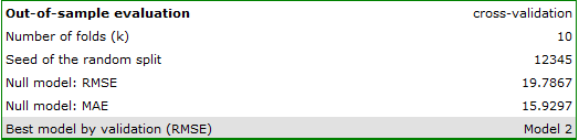
The point of reference is the null model, which assigns to every observation the mean of the dependent variable from the training part – its RMSE and MAE are given in the model selection block of the report. The same block indicates the best model by validation, i.e. the model with the smallest out-of-sample RMSE. It is indicated regardless of the selection criterion chosen, which makes it possible to check whether the model selected, for example, by AIC is also the one that predicts new observations best. Out-of-sample evaluation also works in the manual comparison of models – the report then gives the measures of both models.

If validation error is chosen as the Criterion, the successive selection steps and the marking of the best model are also based on the out-of-sample error. Each model considered is then additionally fitted \(k\) times, so the computations take longer.

Note! When the validation error is the selection criterion, the validation error of the selected model is slightly too optimistic – out of many models, the one that performed best on the given split was chosen (the report gives a note about this). A reliable assessment of the final model can only be obtained from data that took part neither in fitting nor in selecting the model. With small samples, the differences in validation error between models are often smaller than the variability resulting from the random split – it is then worth checking the result for several values of the seed.

How to set up the analysis

Statistics \(\to\) Multivariate models \(\to\) Multiple regression – comparing models.

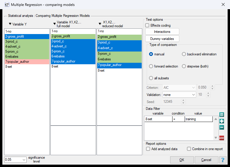
In the window we indicate the dependent variable \(Y\) and the independent variables of the full and the reduced model (in automatic selection – the candidate variables). Model selection options:

Type of comparison – manual or one of the automatic selection methods: backward elimination, forward selection, stepwise (both), all subsets,
Criterion – AIC, AICc, BIC, p (LR / F test) with the threshold given in the adjacent field, or validation error; in the manual mode the criterion is not used,
Validation – none (evaluation on the training set only), k-fold CV, k = with the number of folds in the adjacent field (from 2 to 100, 10 by default) or test set, % = with the share of the test set as a percentage of the observations (from 5 to 90, 30 by default),
Seed – the seed of the random split of the data (12345 by default); the same seed means the same split.

Performing and interpreting the analysis

Continuation of Example 1 (publisher.pqs file): to predict gross profit from book sales, the publisher plans to consider variables such as: production costs, advertising costs, direct promotion costs, the sum of discounts offered, and author's popularity. However, not all of these variables need to have a significant effect on profit. Let us try to choose a linear regression model that will contain the optimal (from a statistical point of view) number of variables. We will use the training set data for this analysis.

Manual comparison of models
Based on the full model built earlier, we might suspect that the variables: direct promotion costs and the sum of discounts offered have little influence on the model being built. We will check whether, from a statistical point of view, the full model is better than the model after removing these two variables.

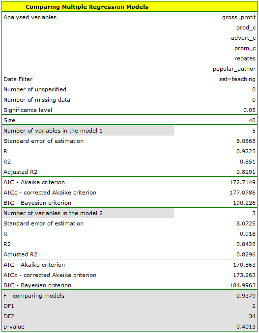
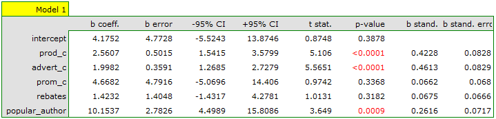
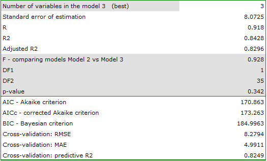
F-test: \(p=0.4013\) (not statistically significant, \(\alpha=0.05\))

There is no reason to think that the full model is better than the reduced model.

Additionally, the reduced model is slightly better fitted than the full model (for the reduced model \(R_{adj}^2=0.8296\), for the full model \(R_{adj}^2=0.8291\)) and has smaller, i.e. more favourable, values of the information criteria AIC, AICc, and BIC.

Automatic model selection
Automatic selection (backward elimination, AIC criterion) gives very similar results. The best model is the one with the highest \(R^2_{adj}\) coefficient, the lowest information criteria, and the lowest standard error of estimation \(SE_e\). The suggested best model here is a model containing only 3 independent variables: production costs, advertising costs, author's popularity.

Out-of-sample evaluation
The comparisons so far were based on the same 40 books on which the models were fitted. We will check whether the choice is confirmed when the models are evaluated on observations that did not take part in fitting them. In the analysis window we keep backward elimination and the AIC criterion, and in the Validation field we choose k-fold CV, k = and enter 10 folds (seed 12345).

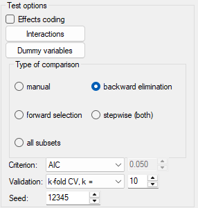
In the model selection block the report gives the method of evaluation, the error of the null model and the best model by validation, and for each model – three rows with the cross-validation measures.

		training set			cross-validation (\(k=10\))
model	variables	\(SE_e\)	\(R^2_{adj}\)	AIC	RMSE	MAE	predictive \(R^2\)
null	0				19.7867	15.9297
Model 1	5	8.0865	0.8291	172.7149	8.3425	5.2976	0.8222
Model 2	4	8.0806	0.8293	171.8163	8.2309	5.1237	0.8270
Model 3	3	8.0725	0.8296	170.8630	8.2794	4.9911	0.8249

Model 1 is the full model, Model 2 was obtained from it by removing direct promotion costs, and Model 3 – by additionally removing the sum of discounts. All three predict the profit many times better than the null model (RMSE of about 8.3 versus 19.8), and the predictive \(R^2\) (0.82–0.83) is only slightly lower than \(R^2_{adj}\) – so the models are not overfitted. At the same time, the out-of-sample error is slightly larger than the standard error of estimation (for Model 3: 8.28 versus 8.07), which was to be expected.

Model 2 has the smallest validation error (RMSE \(=8.2309\)), and Model 3, indicated by AIC, is right behind it (RMSE \(=8.2794\)) and has the smallest mean absolute error (MAE \(=4.9911\)). The differences between these models are negligible compared with the size of the error itself, whereas the full model – although it is the best fitted on the training set (it has the highest \(R^2\)) – predicts new observations the worst of the three (RMSE \(=8.3425\)). Removing direct promotion costs and the sum of discounts therefore does not worsen the predictions, and validation confirms the choice of the model with 3 variables.

cross-validation (\(k=10\)): RMSE \(=8.34\) (Model 1), \(8.23\) (Model 2), \(8.28\) (Model 3); null model: \(19.79\)

The smaller models predict new observations no worse than the full model – the out-of-sample evaluation confirms the choice of the model with 3 variables.

Based on the above analyses, from a statistical point of view, the optimal model is the model containing the 3 most important independent variables: production costs, advertising costs, author's popularity. However, the final decision as to which model to choose belongs to the person with specialist knowledge of the field of study – in this case, the publisher. It should be remembered that the chosen model should be built again and its assumptions verified in the Multiple regression window.

FOR THOSE INTERESTED

Hypotheses:

\(\begin{array}{cc} \mathcal{H}_0: & R_{FM}^2=R_{RM}^2,\\ \mathcal{H}_1: & R_{FM}^2\ne R_{RM}^2, \end{array}\)

where \(R_{FM}^2, R_{RM}^2\) – the multiple coefficients of determination in the compared models (full and reduced).

Formulas: the test statistic is defined by:

\[ F=\frac{R_{FM}^2-R_{RM}^2}{k_{FM}-k_{RM}}\cdot\frac{n-k_{FM}-1}{1-R_{FM}^2}. \]

This statistic has the F Snedecor distribution with \(df_1=k_{FM}-k_{RM}\) and \(df_2=n-k_{FM}-1\) degrees of freedom.

The \(p\) value, determined on the basis of the test statistic, is compared with the significance level \(\alpha\): if \(p \le \alpha\), we reject \(\mathcal{H}_0\) in favor of \(\mathcal{H}_1\); if \(p > \alpha\), there is no reason to reject \(\mathcal{H}_0\).

Out-of-sample evaluation
Let \(\hat{y}_{(-i)}\) denote the value predicted for observation \(i\) by the model fitted without the part of the data to which observation \(i\) belongs (in cross-validation – without its fold, with a test set – on the training set), and \(\overline{y}_{(-i)}\) – the mean of the dependent variable in the same training part. The measures are determined jointly for all the \(n_v\) evaluated observations (in cross-validation – all the observations, with a test set – the observations of the test set):

\[ RMSE=\sqrt{\frac{1}{n_v}\sum_{i=1}^{n_v}\left(y_i-\hat{y}_{(-i)}\right)^2},\qquad MAE=\frac{1}{n_v}\sum_{i=1}^{n_v}\left|y_i-\hat{y}_{(-i)}\right|, \]

\[ R^2_{pred}=1-\frac{\sum_{i=1}^{n_v}\left(y_i-\hat{y}_{(-i)}\right)^2}{\sum_{i=1}^{n_v}\left(y_i-\overline{y}_{(-i)}\right)^2}. \]

The denominator of \(R^2_{pred}\) is the sum of squared errors of the null model, so \(R^2_{pred}\) shows by what part the model reduces the prediction error relative to the null model.

The split: the observations are randomly shuffled (a pseudorandom number generator whose initial state is the seed) and then – in cross-validation – assigned in turn to \(k\) parts whose sizes differ by at most 1; with a test set, the given percentage of the observations (rounded to a whole number) goes to the test set. When \(k\) is greater than the number of observations, \(k\) equal to the number of observations is used. If there are too few observations to set aside a part of the data for validation, the program displays a message.