The McNemar test, the Bowker test of internal symmetry

When to use these tests:

These tests are used when the same feature is measured twice for the same subjects (e.g. an opinion before and after some event), and we want to check whether the results changed. The McNemar test (ang. McNemar test), McNemar (1947)[121], is used when the analysed feature has only 2 categories (denoted (+) and (–)). The Bowker test of internal symmetry (ang. Bowker test of internal symmetry), Bowker (1948)[24], is its extension to features with more than 2 categories (\(c>2\)). Both tests can be calculated on the basis of raw data or a ready-made contingency table.

Assumptions

measurement on a nominal scale – any ordering of categories is not taken into account,
a dependent model.

How to set up the analysis

Statistics \(\to\) NonParametric tests \(\to\) Bowker-McNemar (or via the Wizard).

Step 1. Indicate the two variables corresponding to the first and second measurement of the same feature.

Step 2. Run the analysis.

Note! A common general rule for the validity of the asymptotic McNemar test is the Rufibach condition: the number of discordant pairs should be greater than 10 (\(O_{12}+O_{21}\geq10\))[147]. When this condition is not satisfied, it is better to base the conclusion on the exact probability value of the test (based on the binomial distribution) or on its less conservative version, the mid-p McNemar test[57] – both are calculated automatically together with the basic test.

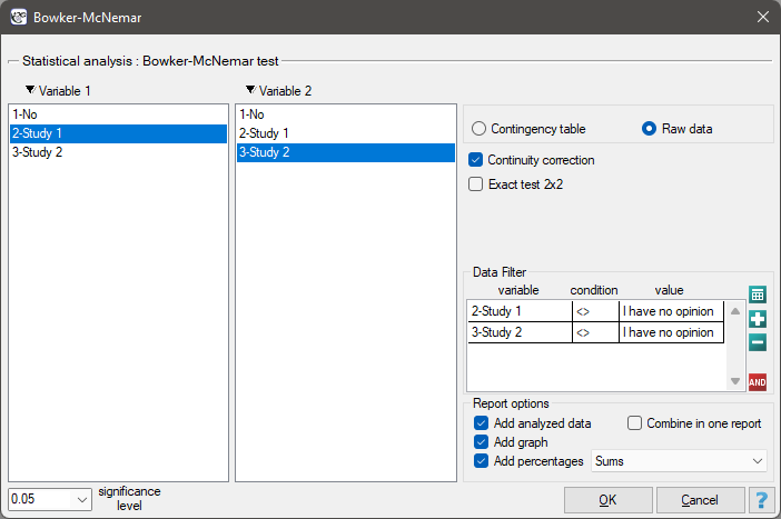
Performance and interpretation

Example 1. (opinion.pqs file)
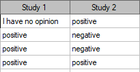
Two surveys of student opinion about a particular academic professor were carried out. Both surveys allowed students to rate the professor negatively, positively, or choose a neutral answer – no opinion. Both surveys were carried out on the same sample of 250 students, with the first survey done the day before the exam in the course taught by the rated professor, and the second the day after the exam. Below is a fragment of the raw data and the complete data as a contingency table. We want to check whether the two surveys give similar results.

\(p<0.0001\) (Bowker test, statistically significant, \(\alpha=0.05\))

Students' opinions about the professor changed between the two surveys.

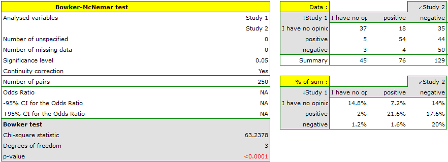
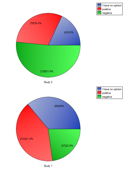
The table shows that significantly more students changed their opinion to negative after the exam than to positive – many students who rated the professor positively before the exam no longer expressed that opinion afterwards.

If we limited the study to people with a defined opinion about the professor (rating him only positively or negatively), we could use the simpler McNemar test:

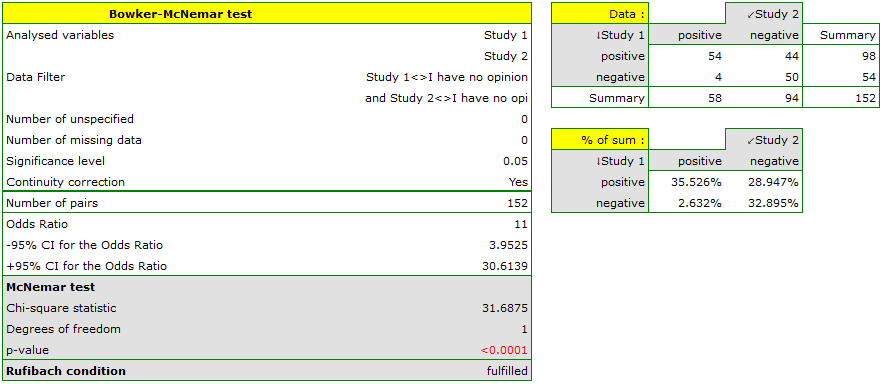
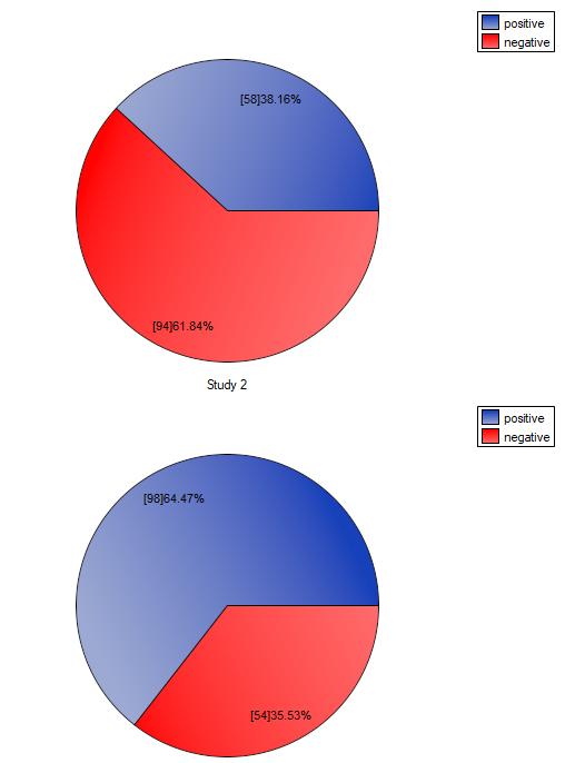
\(p<0.0001\) (McNemar test, statistically significant, \(\alpha=0.05\))

Among students with a clear-cut opinion, its distribution (positive/negative) changed between the two surveys.

Significantly more students changed their opinion to negative after the exam than to positive. The odds of changing an opinion from positive (before the exam) to negative (after the exam) are eleven times greater (\(\frac{44}{4}\)) than the odds of changing in the opposite direction (\(\frac{4}{44}\)).

Definitions of measures

Odds ratio (OR) (ang. odds ratio) – if a study of the same feature on the same objects was carried out twice, the odds ratio describes how many times more (or less) likely a change of result in one direction (e.g. from (+) to (–)) is than a change in the opposite direction.

FOR THOSE INTERESTED

Notation:
Notation for the \(2\times 2\) contingency table for McNemar's test:

Observed frequencies		\(X^{(2)}\)
\(O_{ij}\)		(+)	(–)	Total
\(X^{(1)}\)	(+)	\(O_{11}\)	\(O_{12}\)	\(O_{11}+O_{12}\)
	(–)	\(O_{21}\)	\(O_{22}\)	\(O_{21}+O_{22}\)
	Total	\(O_{11}+O_{21}\)	\(O_{12}+O_{22}\)	\(n=O_{11}+O_{12}+O_{21}+O_{22}\)

The McNemar test – hypotheses:

\(\begin{array}{cl} \mathcal{H}_0: & O_{12}=O_{21}, \\ \mathcal{H}_1: & O_{12}\neq O_{21}. \end{array}\)

Formulas:
The test statistic is defined by:

\[ \chi^2=\frac{(O_{12}-O_{21})^2}{O_{12}+O_{21}}. \]

This statistic asymptotically (for large frequencies) has the \(\chi^2\) distribution with 1 degree of freedom.

Continuity correction for the McNemar test is more conservative than the basic test (it rejects the null hypothesis more rarely). The test statistic with the correction is defined by:

\[ \chi^2=\frac{(|O_{12}-O_{21}|-1)^2}{O_{12}+O_{21}}. \]

Odds ratio of a result change – if the same feature was measured twice on the same objects, for such a table we calculate the odds ratio for a result change (from (+) to (–) and vice versa). The odds of a change from (+) to (–) is \(O_{12}\), and from (–) to (+) is \(O_{21}\). The odds ratio is calculated using the formula:

\[ OR=\frac{O_{12}}{O_{21}}. \]

The confidence interval for the odds ratio is built on the basis of the standard error:

\[ SE=\sqrt{\frac{1}{O_{12}}+\frac{1}{O_{21}}}. \]

For samples with small frequencies, the exact range of the confidence interval for the odds ratio can additionally be determined[105].

The Bowker test of internal symmetry extends the McNemar test to \(c\times c\) tables (\(c>2\) categories):

Observed frequencies		\(X^{(2)}\)
\(O_{ij}\)		\(X_1^{(2)}\)	\(X_2^{(2)}\)	...	\(X_c^{(2)}\)	Total
\(X^{(1)}\)	\(X_1^{(1)}\)	\(O_{11}\)	\(O_{12}\)	...	\(O_{1c}\)	\(\sum_{j=1}^cO_{1j}\)
	\(X_2^{(1)}\)	\(O_{21}\)	\(O_{22}\)	...	\(O_{2c}\)	\(\sum_{j=1}^cO_{2j}\)
	...	...	...	...	...	...
	\(X_c^{(1)}\)	\(O_{c1}\)	\(O_{c2}\)	...	\(O_{cc}\)	\(\sum_{j=1}^cO_{cj}\)
	Total	\(\sum_{i=1}^cO_{i1}\)	\(\sum_{i=1}^cO_{i2}\)	...	\(\sum_{i=1}^cO_{ic}\)	\(n=\sum_{i=1}^c\sum_{j=1}^cO_{ij}\)

Hypotheses (where \(j\neq i\), \(j,i\in\{1,2,...,c\}\), and \(O_{ij}\) and \(O_{ji}\) are the frequencies of symmetric pairs):

\[\begin{array}{cl} \mathcal{H}_0: & O_{ij}=O_{ji},\\ \mathcal{H}_1: & O_{ij}\neq O_{ji} \text{ for at least one pair } O_{ij}, O_{ji}. \end{array}\]

Formulas:
The test statistic is defined by:

\[ \chi^2=\sum_{i=1}^c\sum_{j>i}\frac{(O_{ij}-O_{ji})^2}{O_{ij}+O_{ji}}. \]

This statistic asymptotically (for large sample sizes) has the \(\chi^2\) distribution with a number of degrees of freedom calculated using the formula \(df=\frac{c(c-1)}{2}\).