The Fisher test for large tables

When to use this test:

The Fisher test for \(r\times c\) tables, also called the Fisher-Freeman-Halton test (ang. Fisher-Freeman-Halton test), Freeman G.H., Halton J.H. (1951)[65], is used instead of the \(\chi^2\) test for \(r\times c\) tables when the expected frequencies in the table are too small (Cochran's condition is not satisfied). It is an extension to \(r\times c\) tables of the Fisher exact test, determining the exact probability of the occurrence of a particular distribution of numbers in the table, given a known \(n\) and fixed marginal sums.

Assumptions

measurement on a nominal scale,
an independent model,
small expected frequencies (the \(\chi^2\) test is not advisable).

How to set up the analysis

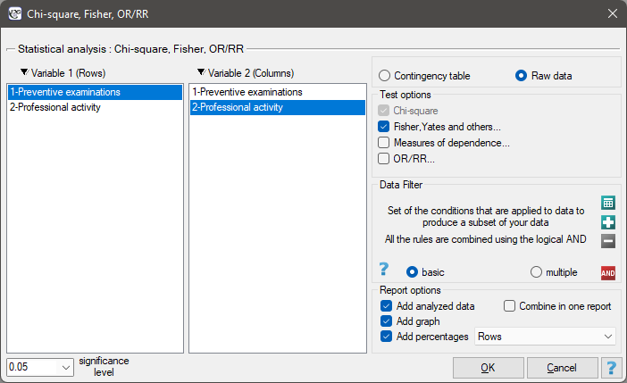
Statistics \(\to\) NonParametric tests \(\to\) Chi-square, Fisher, OR/RR (or via the Wizard).

Step 1. Indicate the two features whose dependence you want to check.

Step 2. Run the analysis.

Note! The procedure for calculating the \(p\) value for this test is based on the algorithm published by Mehta (1986)[122].

Performance and interpretation

Example 1. (job-prevention.pqs file)
In the population of people living in the rural areas of Komorniki municipality, it was examined whether performing preventive health examinations depends on the type of occupational activity of the residents. A random sample of 120 people was collected and asked about their education and whether they perform preventive examinations. Complete answers were obtained from 113 people.

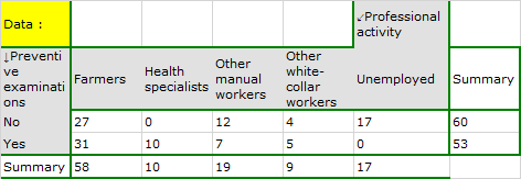
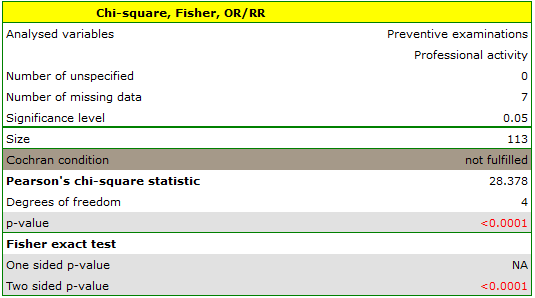
\(p<0.0001\) (Fisher test, statistically significant, \(\alpha=0.05\))

There is a dependence between performing preventive examinations and the type of work performed, in the analysed population.

Cochran's condition is not satisfied, so we should not use the chi-square test – hence the choice of the Fisher test. If we are interested in more precise information about the detected dependence, we can obtain it by determining multiple comparisons through the Fisher, Yates and others... option, then Multiple column comparisons (RxC) and one of the corrections, e.g. Benjamini-Hochberg.

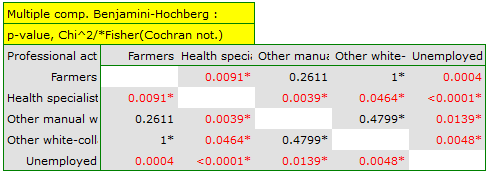
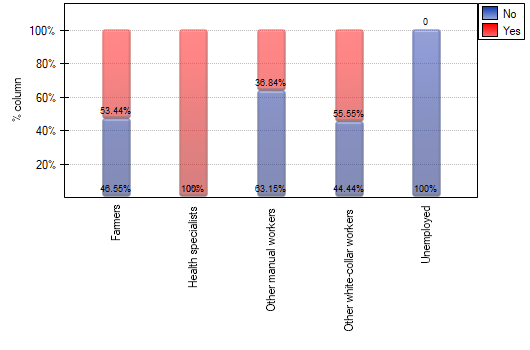
A closer analysis allows us to conclude that health professionals perform preventive examinations significantly more often than the other groups (100% of people in this group performed examinations), and the unemployed significantly less often (no one in this group performed an examination). Farmers, other manual workers, and other white-collar workers take preventive examinations in about 50% of cases, which means these three groups do not differ from each other in a statistically significant way. \(p\) values in the table marked with an asterisk come from the Fisher exact test with the Benjamini-Hochberg correction, while unmarked values come from the chi-square test with the same correction (where Cochran's condition was satisfied).

FOR THOSE INTERESTED

Hypotheses:

\[ \begin{array}{cl} \mathcal{H}_0: & \text{there is no dependence between the analysed features in the population,}\\ \mathcal{H}_1: & \text{there is a dependence between the analysed features in the population.} \end{array} \]

Formulas: Marginal row sums are defined as:

\[ W_i=\sum_{j=1}^cO_{ij}, \]

where \(O_{ij}\) – observed frequencies in a contingency table, and marginal column sums as:

\[ K_i=\sum_{i=1}^rO_{ij}. \]

Given fixed marginal sums, for various configurations of observed frequencies denoted as \(U_{ij}\), we calculate the probabilities \(P\):

\[ P=\frac{D^{-1}\prod_{j=1}^{c}K_j!}{U_{1j}!U_{2j}!\dots U_{rj}}, \]

where

\[ D=\frac{(W_1+W_2+\dots+W_r)!}{W_1!W_2!\dots W_r!}. \]

Interpretation: The exact significance level \(p\) is the sum of those \(P\) probabilities (calculated for new values \(U_{ij}\)) that are less than or equal to the \(P\) probability of the table with the initial values \(O_{ij}\).