 PQStat
The Z test for two dependent proportions
When to use this test:
The \(Z\) test for two dependent proportions is used when the same feature with two possible outcomes (e.g. yes/no, agree/disagree) is measured twice for the same subjects, and we want to check whether the share of one of the outcomes changed between the measurements (e.g. before and after some event). This is a similar situation to the McNemar test.
Assumptions
- measurement on a nominal scale – any ordering of categories is not taken into account,
- a dependent model,
- large sample size.
How to set up the analysis
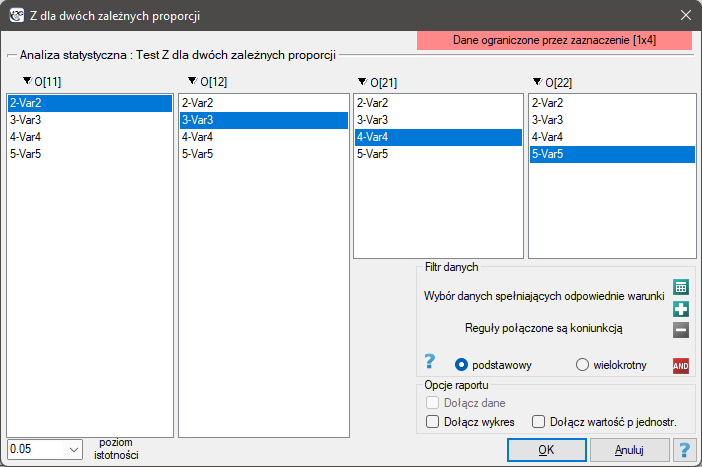
Statistics \(\to\) NonParametric tests \(\to\) Z for 2 dependent proportions.
Performance and interpretation
Example 1. Example (1) cont. (opinion.pqs file)
If we limit the study to people with a defined opinion about the professor (rating him only positively or negatively), we obtain 152 such students. Among them: 50 students rated the professor positively both before and after the exam; 4 students rated him well before the exam, but poorly after the exam; 44 students rated him poorly before the exam, but well after the exam; 54 students rated him negatively both before and after the exam. So we know that \(\frac{50+4}{152}=35.53\%\) of students expressed a negative opinion before the exam, and after the exam the corresponding percentage was \(\frac{50+44}{152}=61.84\%\). We want to check whether the proportion of negative ratings changed between the measurements.
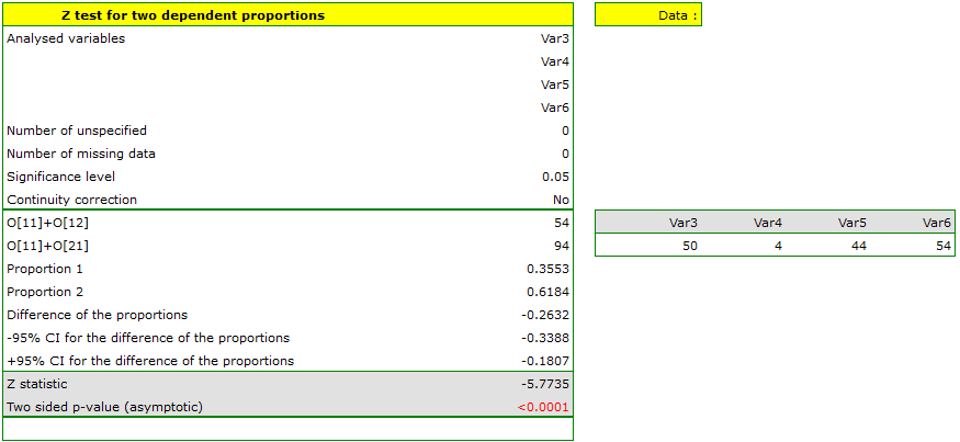
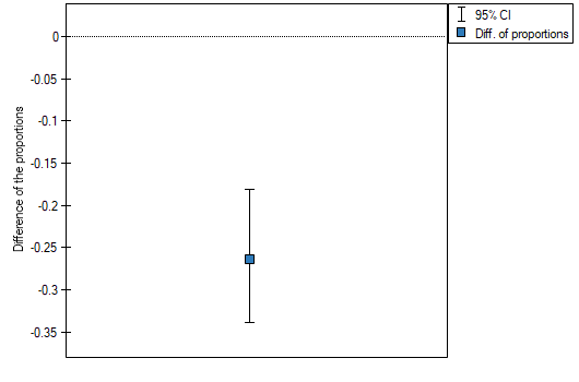
The difference between the proportions distinguished in the sample is 26.32%, and its 95% confidence interval \((18.07\%, 33.88\%)\) does not contain 0 – the same conclusion is reached by the McNemar test. After the exam, the professor is rated negatively significantly more often.
Definition: Notation for the contingency table of two dependent measurements of the same feature \(X\) (first measurement \(X^{(1)}\), second measurement \(X^{(2)}\)), each with two possible outcomes (+) and (–):
| Observed frequencies | \(X^{(2)}\) | |||
| \(O_{ij}\) | (+) | (–) | Total | |
| \(X^{(1)}\) | (+) | \(O_{11}\) | \(O_{12}\) | \(O_{11}+O_{12}\) |
| (–) | \(O_{21}\) | \(O_{22}\) | \(O_{21}+O_{22}\) | |
| Total | \(O_{11}+O_{21}\) | \(O_{12}+O_{22}\) | \(n=O_{11}+O_{12}+O_{21}+O_{22}\) | |
where \(O_{11}\) – the number of people with a (+) outcome in both measurements, \(O_{12}\) – the number of people who changed outcome from (+) to (–), \(O_{21}\) – the number of people who changed outcome from (–) to (+), \(O_{22}\) – the number of people with a (–) outcome in both measurements.
For these data we calculate the distinguished proportions \(p_1=\frac{O_{11}+O_{12}}{n}\) and \(p_2=\frac{O_{11}+O_{21}}{n}\).
Hypotheses:
\( \begin{array}{cl} \mathcal{H}_0: & P_1-P_2=0,\\ \mathcal{H}_1: & P_1-P_2\neq 0, \end{array} \)
where \(P_1\), \(P_2\) – distinguished proportions in the population, for the first and second measurement.
Formulas: The test statistic is defined by:
and asymptotically (for large sample sizes) has the normal distribution.