Life tables

Survival analysis allows us to evaluate how long it takes for an event of interest to a researcher to occur – e.g. how long patients live after surgery, how long a disease remission lasts, or after what time a device fails. Outside medicine (where the name originates) it is also used in other fields, where it goes by other names: reliability analysis, duration analysis, or event history analysis.
The basic descriptive tools here are life tables and Kaplan-Meier curves, which allow us to estimate what proportion of the study group „survives” up to a given point in time. When we are interested in comparing survival time between groups (e.g. between different treatment methods), we use the comparison of survival curves. The influence of many variables at once on survival time is studied by means of regression models, primarily Cox proportional hazard regression.
The basic concepts of survival analysis will be explained using the example of the life expectancy of heart transplant patients:

Event – a change of interest to the researcher, e.g. death.
Survival time – the period that elapses between the initial state and the occurrence of the event, e.g. the length of a patient's life after a heart transplantation.

Note! One column with the ready-made, calculated time should be prepared for the analysis. When we have two dates at our disposal – an initial and a final one – the elapsed time between them should be calculated before the analysis, using worksheet formulas.
Censored observations – observations for which we do not have complete information about survival time. We distinguish here:
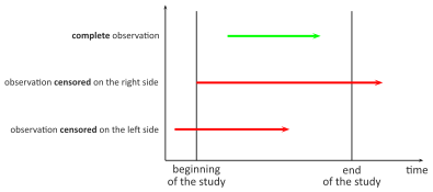
- a complete observation – both the date of the transplantation and the date of the patient's death are known, so the exact survival time after the transplantation can be determined;
- an observation censored on the right – the date of the patient's death is not known (the patient is still alive when the study ends), so the exact survival time cannot be determined;
- an observation censored on the left – the date of the heart transplantation is not known, although it is known to have occurred before the study began, so here too the exact survival time cannot be determined.

Note! The end of the study means the end of observation of a given patient – it is not always the same moment for all subjects. The end of observation can be, for example, the moment when contact with the patient is lost (so we no longer know their further survival time). Similarly, the start of the study does not have to occur at the same time for all patients.

When to use:

Life tables (survival tables) are the simplest way of summarizing the survival time of a study group – the timeline is divided into equal intervals (e.g. every 3 years), and for each of them we check how many subjects survived to it, how many died, and how many were lost to follow-up (censored). Their advantage is ease of interpretation; their drawback is the need to arbitrarily divide time into intervals.

Definitions of measures

For each time interval PQStat calculates:

the number of entering cases – the number of people who survived to the beginning of the given interval;
the number of censored cases – the number of people in a given interval defined as censored cases;
the number of cases at risk – the number of cases entering the given interval reduced by half of the number of censored cases in that interval;
the number of complete cases – the number of people who experienced the event (e.g. died) in a given interval;
the proportion of complete cases – the ratio of the number of complete cases (deaths) in a given interval to the number of cases at risk in that interval;
the proportion of surviving cases – calculated as 1 minus the proportion of complete cases in a given interval;
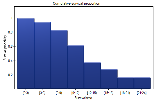
the cumulative survival proportion (survival function) – the probability of surviving up to a given time; since surviving another interval requires having survived all the previous ones, this probability is calculated as the product of all the previous proportions of surviving cases

\(\pm\) the standard error of the survival function;
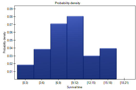
probability density – the estimated probability of experiencing the event (death) in a given interval, expressed per unit of time

\(\pm\) the standard error of the probability density;
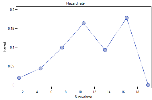
the hazard rate – the probability (per unit of time) that a case which survived to the beginning of a given interval will experience the event (die) precisely in that interval

\(\pm\) the standard error of the hazard rate.

Note! When there is no complete observation in some interval of survival time, the program allows the use of a correction – the zero number of complete cases is then replaced with the value 0.5.

The information obtained can be illustrated with three graphs: a graph of the survival function, a graph of the probability density, and a graph of the hazard rate.

How to set up the analysis

The window with the settings for life tables is accessed via the menu Statistics\(\to\)Survival analysis\(\to\)Life tables.

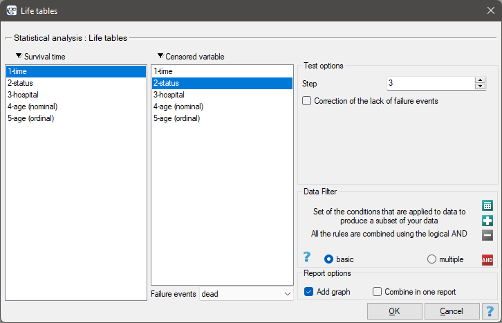
Life tables are built for survival-time intervals of equal width, given by the researcher – these intervals are defined by specifying their step.

Calculation and interpretation

Example 1. (transplant.pqs file)
Patients' survival after liver transplantation was studied. A group of 89 patients was observed over 21 years; their age at the time of the transplantation ranged from \(\langle 45 \)years\(; 60 \)years\()\). A fragment of the collected data is presented in the table below:

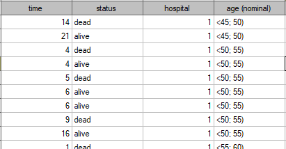
The complete data in this analysis are those for which we have full information about the length of life after the transplantation, i.e. described as „death” (53 people, i.e. 59.55%). The censored data are those for which we lack that information because the patients were still alive when the study ended (36 people, i.e. 40.45%). We build life tables for these patients, creating 3-year time intervals:

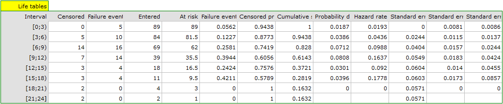
For each 3-year interval we can interpret the results obtained in the table – for example, for people who lived at least 9 years after the transplantation, i.e. who entered the interval [9;12):

the number of people who survived to 9 years after the transplantation is 39;
there are 7 people we know lived at least 9-12 years – information about them was collected, but we do not know whether they lived longer, since they were lost to the study after this time;
the number of people at risk of death in this interval is 36;
there are 14 people we know died 9 to 12 years after the transplantation;
39.4% of the endangered patients died 9-12 years after the transplantation;
60.6% of the endangered patients lived 9-12 years after the transplantation;
the percentage surviving to 9 years after the transplantation is 61.4% \(\pm\) 5%;
0.08 \(\pm\) 0.02 – the probability of death for each year of the 9-12 interval;
0.16 \(\pm\) 0.04 – the conditional, annual probability of death for a case that survived to the beginning of the 9-12 interval.

We will present the results on a few graphs:

The survival function declines gradually, without a sudden drop

The probability of survival decreases with the time elapsed since the transplantation, but we do not observe a period in which the probability of death would rise sharply.

Kaplan-Meier curves

When to use:

Kaplan-Meier curves allow the evaluation of survival time without the need to arbitrarily group observations into intervals, as is the case with life tables. This estimator was introduced by Kaplan and Meier (1958)[93]. The graph of the Kaplan-Meier survival function has the form of a step function.

Definitions of measures

As with life tables, we calculate here the survival function, i.e. the probability of survival up to a given time. Confidence intervals around this curve are constructed on the basis of the standard error (Greenwood's formula) and a logarithmic transformation (log-log).
The point in time at which the value of the function equals 0.5 is the survival time median. This median indicates a 50% risk of death, i.e. it predicts that half of the patients will die within the indicated time. Both the median and other percentiles are determined as the shortest survival time for which the survival function is less than or equal to the given percentile. For the median, a confidence interval is determined using the „test-based” method of Brookmeyer and Crowley (1982)[30].
The survival time mean is determined as the area under the survival curve. Data concerning survival time are usually strongly skewed, which is why in survival analysis the median is usually a better measure of central tendency than the mean.

How to set up the analysis

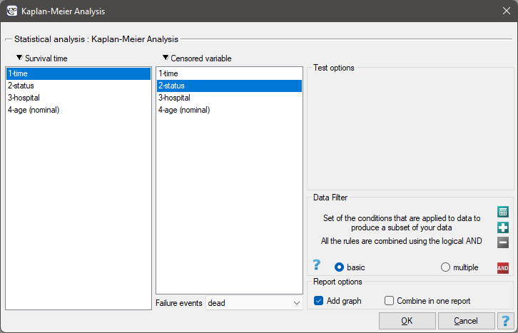
The window with the settings for the Kaplan-Meier curve is accessed via the menu Statistics\(\to\)Survival analysis\(\to\)Kaplan-Meier Analysis.

Calculation and interpretation

Example (1) continued (transplant.pqs file)
We present the survival time after a liver transplantation using the Kaplan-Meier curve:

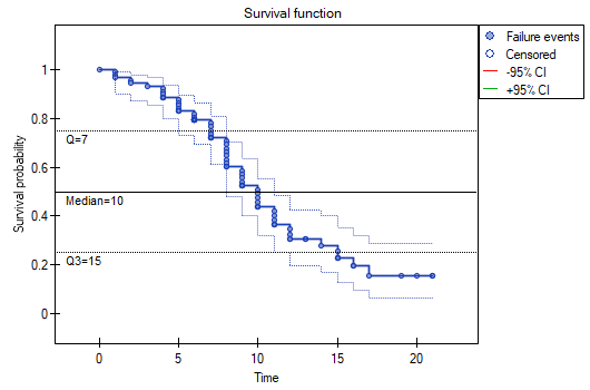
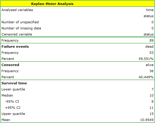
The survival function does not drop sharply right after the transplantation. We conclude from this that the initial period after transplantation does not carry a particular risk of death.

Median survival time \(=10\) years

Within 10 years of the transplantation we expect that death will occur in half of the patients. This value is marked on the graph by drawing a line at the point 0.5 corresponding to the median. The quartiles are marked on the graph in a similar way.

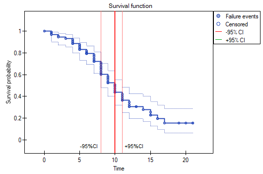
We can visualize the confidence interval for the median on the graph by drawing vertical lines based on the confidence interval around the curve and a line at the 0.5 level.

Comparison of survival curves

When to use:

Survival functions can be constructed separately for different subgroups, e.g. separately for women and men, and then compared with one another. Such a comparison may concern two or several curves at once; it can also examine whether the curves follow a natural trend (e.g. with age), and can adjust (correct) the analysis for the effect of an additional factor (a stratum).
A comparison of \(k\) survival curves \(S_1,S_2,\ldots,S_k\) can be made in the program with the use of three tests:

the log-rank test – the best-known and most widely used, drawing on the Mantel-Haenszel procedure for many 2\(\times\)2 tables (Mantel-Haenszel 1959[114], Mantel 1966[116], Cox 1972[49]),
Gehan's generalization of the Wilcoxon test – derived from the Wilcoxon test (Breslow 1970, Gehan 1965[70][71]),
the Tarone-Ware test – derived from the Wilcoxon test (Tarone and Ware 1977[161]).

All three tests are based on the same test statistic – they differ only in the weights \(w_j\) assigned to particular points on the timeline:

the log-rank test: \(w_j=1\) – all points on the timeline have the same weight, which gives later values of the timeline a greater influence on the result;
Gehan's generalization of the Wilcoxon test: \(w_j=n_j\) – time points are weighted by the number of observations at each of them, so the initial values of the timeline carry greater weight;
the Tarone-Ware test: \(w_j=\sqrt{n_j}\) – time points are weighted by the square root of the number of observations, which situates this test between the two above.

Assumptions

hazard proportionality – hazard, defined as the slope of the survival curve, is a measure of how quickly the event of interest occurs; violating this assumption does not entirely disqualify the tests above, but it lowers their power, the more so the earlier on the timeline the curves cross.

Definitions of measures

The Hazard Ratio (\(HR\)) describes the magnitude of the observed difference between a pair of survival curves, on the basis of the number of events observed and expected in each group:

\[ HR= \frac{O_1/E_1}{O_2/E_2} \]

If \(HR>1\) (e.g. \(HR=2\)), the degree of exposure to the event of interest in the first group is correspondingly greater than in the second group (twice as great for \(HR=2\)); if \(HR<1\), the situation is reversed; \(HR\approx1\) means that both groups are exposed to a similar degree.

Note! The confidence interval for \(HR\) is calculated on the basis of the standard error of the logarithm of \(HR\) (Armitage and Berry 1994[11]).

The program also allows us to check whether the curves follow a trend consistent with the natural order of the compared groups (e.g. successive age categories), and to compare curves taking strata into account, i.e. after adjusting for an additional factor which may affect the result of the comparison (e.g. when comparing survival time with respect to age, separately within strata defined by sex).

How to set up the analysis

The window with the settings for the comparison of survival curves is accessed via the menu Statistics\(\to\)Survival analysis\(\to\)Comparison of groups.

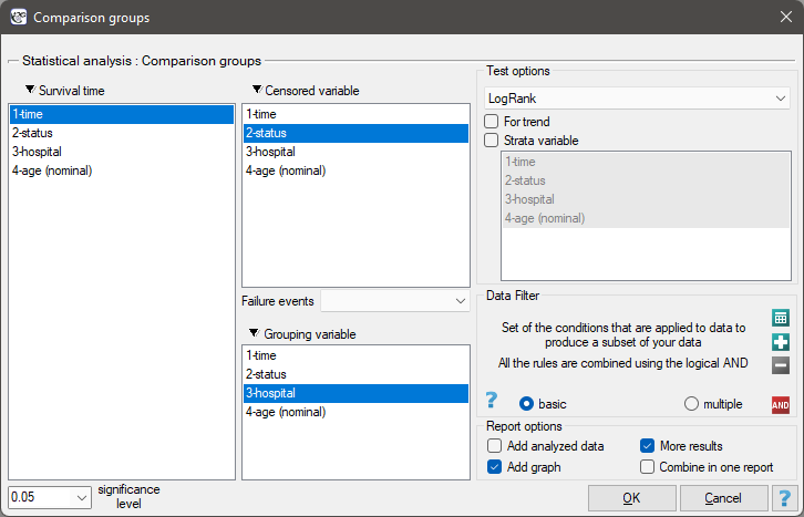
Calculation and interpretation

Example (1) continued (transplant.pqs file)
Differences between two survival curves
Liver transplantations were performed in two different hospitals. We will check whether patients' survival time after transplantation depended on the hospital in which the transplantation was performed. The comparison of the survival curves for these hospitals will be made using all the tests offered by the program for this purpose.
Hypotheses:

\[\begin{array}{ll} \mathcal{H}_0: & \text{the survival curve of hospital 1 patients }=\text{ the survival curve of hospital 2 patients},\\ \mathcal{H}_1: & \text{the survival curve of hospital 1 patients }\neq \text{ the survival curve of hospital 2 patients}. \end{array}\]

\(p=0.6004\) for the log-rank test (\(p=0.6959\) for Gehan's, \(p=0.6465\) for Tarone-Ware); \(HR=1.1499\), 95%CI: \(\langle\)0.6570; 2.0126\(\rangle\)

There is no reason to reject \(\mathcal{H}_0\) – the length of life of the patients in both hospitals is similar (the confidence interval for \(HR\) contains the value 1).

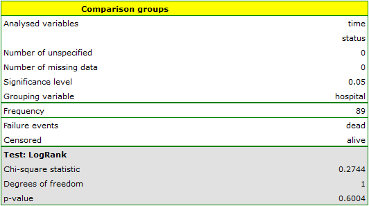
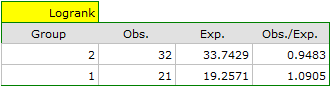
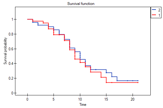
Differences among several survival curves
Liver transplantations were performed on people of different ages. Three age groups were distinguished: \(\langle 45 \)years\(; 50 \)years\()\), \(\langle 50 \)years\(; 55 \)years\()\), \(\langle 55 \)years\(; 60 \)years\()\). We will check whether patients' survival time after transplantation depends on their age at the time of the transplantation.
Hypotheses:

\[\begin{array}{ll} \mathcal{H}_0: & \text{the survival curves of patients aged }\langle 45 \text{years}; 50 \text{years}), \langle 50 \text{years}; 55 \text{years}), \langle 55 \text{years}; 60 \text{years})\\ & \text{are similar,}\\ \mathcal{H}_1: & \text{at least one survival curve, out of the 3 curves above,}\\ & \text{differs from the others.}\\ \end{array}\]

\(p=0.0692\) for the log-rank test (\(p=0.0928\) for Gehan's, \(p=0.0779\) for Tarone-Ware)

There is no reason to reject \(\mathcal{H}_0\) – the length of life of the patients from the three age groups is similar, although the \(p\) values are quite close to the significance level of 0.05.

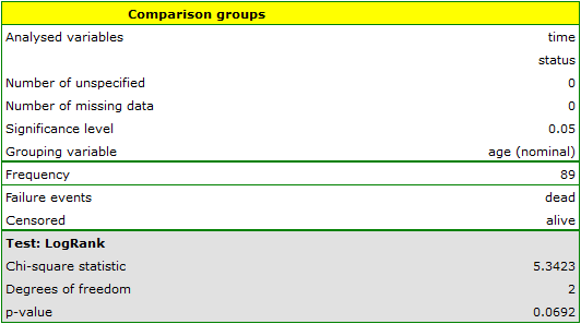
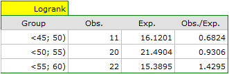
Looking at the hazard values (the ratio of observed to expected events), we notice that they are slightly higher with each successive age group: \(\langle\)0.68, 0.93, 1.43\(\rangle\). Although these differences are not statistically significant, they may suggest the existence of a trend of increasing hazard with age.
Trend among several survival curves
By introducing into the test information about the ordering of the compared categories (using the age variable, in which the age ranges are numbered 1, 2, and 3, respectively), we will check whether there is a trend in the compared curves.
Hypotheses:

\[\begin{array}{ll} \mathcal{H}_0: & \text{there is no trend in the survival time curves of patients after transplantation}\\ & \text{(a trend dependent on patients' age at the time of the transplantation),}\\ \mathcal{H}_1: & \text{the older the patients at the time of the transplantation, the greater/smaller}\\ & \text{the probability of their survival over a given period of time.}\\ \end{array}\]

\(p=0.0237\) for the log-rank test (\(p=0.0317\) for Gehan's, \(p=0.0241\) for Tarone-Ware)

The survival curves are arranged in a statistically significant trend: the older the patient at the time of the transplantation, the smaller the probability of surviving a given period of time.

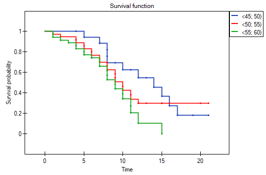
The lowest curve on the Kaplan-Meier graph is that for people aged \(\langle\)55 years; 60 years); above it is the curve for patients aged \(\langle\)50 years; 55 years), and the highest curve is that for patients aged \(\langle\)45 years; 50 years).
Survival curves for strata
We will now check whether the trend observed earlier is independent of the hospital in which the transplantation was performed. For this purpose we will choose hospital as the stratum variable.

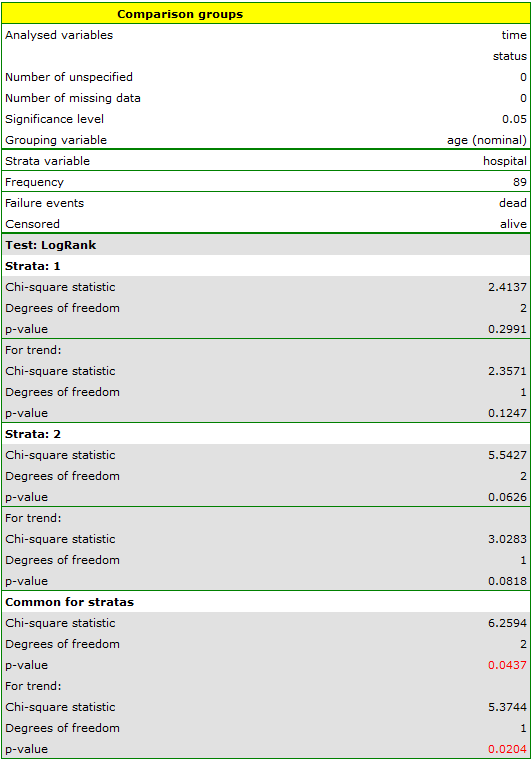
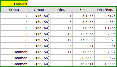
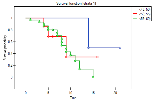
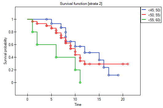
The report first presents an analysis of the individual strata, both the test results and the hazard values. In the first stratum an increasing trend in hazard is visible, though not statistically significant; a trend in the same direction (bordering on significance) is observed in the second stratum. Pooling these trends in a joint stratified analysis allowed us to obtain a significant trend in the survival curves.

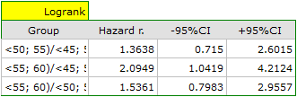
Stratified analysis: the trend is significant regardless of hospital

The older the patient at the time of the transplantation, the smaller the probability of surviving a given period of time – regardless of the hospital where the transplantation was performed.

A comparative analysis of the survival curves, adjusted for strata, gives a significant result for the log-rank and Tarone-Ware tests and a non-significant result for Gehan's test, which may indicate that the differences between the curves are not as visible in the early periods of survival time as in the later ones. Looking at the hazard ratio for the curves compared in pairs

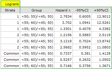
we can localize the significant differences. The smallest hazard ratio was obtained for the comparison of the curve for the youngest group with the curve for the oldest group: 0.53; the 95% confidence interval \(\langle\)0.26; 1.05\(\rangle\) does contain the value 1, but is close to it, which may suggest significant differences between the corresponding curves. To confirm this supposition, the data filter in the analysis window can be used to compare the curves pairwise.

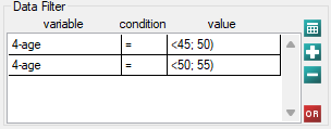
Note! For pairwise comparisons, one of the corrections used for multiple comparisons should be applied and the significance level modified. Here, with Bonferroni's correction for three comparisons, the significance level will be 0.017. For simplicity we will use only the log-rank test.

\(\langle\)45 years; 50 years) vs \(\langle\)50 years; 55 years)

\(\langle\)45 years; 50 years) vs \(\langle\)55 years; 60 years)

\(\langle\)50 years; 55 years) vs \(\langle\)55 years; 60 years)

As expected, statistically significant differences concern only the survival curves for the youngest and oldest age groups.

FOR THOSE INTERESTED

Differences among survival curves
Hypotheses:

\[\begin{array}{ll} \mathcal{H}_0: & S_1(t)=S_2(t)=...=S_k(t),\text{for all }t,\\ \mathcal{H}_1: & \text{not all }S_i(t)\text{ are equal}. \end{array}\]

Formulas:

Test statistic (chi-square):

\[ \chi^2=U'V^{-1}U \]

where:

\(U_i=\sum_{j=1}^{m}w_j(d_{ij}-e_{ij})\),
\(V\) – the covariance matrix of dimensions \((k-1)\times(k-1)\):

diagonal: \(\sum_{j=1}^{m}w_j^2\frac{n_{ij}(n_j-n_{ij})d_j(n_j-d_j)}{n^2_j(n_j-1)}\),
off-diagonal: \(\sum_{j=1}^{m}w_j^2\frac{n_{ij}n_{lj}d_j(n_j-d_j)}{n^2_j(n_j-1)}\),

\(m\) – the number of time points at which the event of interest (death) occurred,
\(d_j=\sum_{i=1}^k d_{ij}\) – the observed number of events in the \(j\)-th time point,
\(d_{ij}\) – the observed number of events in the \(i\)-th group in the \(j\)-th time point,
\(e_{ij}=\frac{n_{ij}d_j}{n_j}\) – the expected number of events in the \(i\)-th group in the \(j\)-th time point,
\(n_j=\sum_{i=1}^k n_{ij}\) – the number of cases at risk in the \(j\)-th time point.

This statistic asymptotically (for large expected counts) has the \(\chi^2\) distribution with \(df=k-1\) degrees of freedom.

The \(p\) value, determined on the basis of the test statistic, is compared with the significance level \(\alpha\): if \(p \le \alpha\), we reject \(\mathcal{H}_0\) in favor of \(\mathcal{H}_1\); if \(p > \alpha\), there is no reason to reject \(\mathcal{H}_0\).

Trend among survival curves
Hypotheses:

\[\begin{array}{ll} \mathcal{H}_0: & \text{there is no trend, in the studied population, in the placement of curves }S_1,S_2,...,S_k,\\ \mathcal{H}_1: & \text{there is a trend, in the studied population, in the placement of curves }S_1,S_2,...,S_k. \end{array}\]

Formulas:

Test statistic (chi-square):

\[ \chi^2=\frac{(c'U)^2}{c'Vc} \]

where \(c=(c_1,c_2,...,c_k)\) – a vector of weights for the compared groups, informing about their natural order (usually consecutive natural numbers). This statistic asymptotically (for large expected counts) has the \(\chi^2\) distribution with one degree of freedom.

Note! To be able to perform a trend analysis in the survival curves, the grouping variable must be a numerical variable whose values indicate the natural order of the groups – these numbers are treated in the analysis as the weights \(c_1,c_2,...,c_k\).

Survival curves for strata
Hypotheses for differences among survival curves:

\[\begin{array}{ll} \mathcal{H}_0: & S_1^*(t)=S_2^*(t)=...=S_k^*(t),\text{for all }t,\\ \mathcal{H}_1: & \text{not all }S_i^*(t)\text{ are equal}. \end{array}\]

Hypotheses for the trend analysis in survival curves:

\[\begin{array}{ll} \mathcal{H}_0: & \text{there is no trend, in the studied population, in the placement of curves }S_1^*,S_2^*,...,S_k^*,\\ \mathcal{H}_1: & \text{there is a trend, in the studied population, in the placement of curves }S_1^*,S_2^*,...,S_k^*, \end{array}\]

where \(S_1^*(t), S_2^*(t), ..., S_k^*(t)\) – the survival curves after adjustment for the variable defining the strata. The calculations for the test statistics are based on the formulas described for the tests without strata, with the difference that matrices \(U\) and \(V\) are replaced with the sums of matrices \(\sum_{l=1}^L U\) and \(\sum_{l=1}^L V\), summed over the strata created by the adjusting variable (\(l=1,2,...,L\)).

Cox proportional hazards regression

When to use:

Cox regression, also known as the Cox proportional hazards model (Cox PH model) – Cox D.R. (1972)[49], is the most widely used regression approach in survival analysis. It allows the study of the simultaneous influence of many independent variables (\(X_1\), \(X_2\), \(\ldots\), \(X_k\)) on survival time, e.g. the influence of the treatment method, age and other prognostic factors on lifetime. It is, in a sense, a non-parametric approach – it does not require knowledge of the shape of the hazard or survival function, which is the source of its popularity.

Assumptions

hazard proportionality – the effect of each independent variable on the hazard must be constant over time (see Analysis of model residuals below);
no strong collinearity of the independent variables;
a sufficiently large number of observations relative to the number of estimated parameters.

Note! The number of observations should be at least ten times greater than the ratio of the number of estimated model parameters (\(k\)) to the smaller of the proportions of censored or complete observations (\(p\)), i.e. \(n\ge 10k/p\) (Peduzzi et al. 1995[134]).

Note! The independent variables should not be collinear – collinearity leads to uncertain estimation and very high values of the errors.

Definitions of measures

The function on which the model is based describes the resulting hazard as the product of two quantities, only one of which depends on time (\(t\)):

\[ h(t,X_1,X_2,...,X_k)=h_0(t)\cdot \exp\left(\sum_{i=1}^k\beta_iX_i\right), \]

where \(h(t,X_1,...,X_k)\) is the resulting hazard (the risk changing over time, depending on other factors, e.g. the treatment method), \(h_0(t)\) is the baseline hazard (the hazard assuming that all explanatory variables are equal to zero), and \(\sum_{i=1}^k\beta_iX_i\) is a (usually linear) combination of the independent variables \(X_1,...,X_k\) and the model parameters \(\beta_1,...,\beta_k\), called regression coefficients. The preparation of dummy variables and interactions is discussed in chapter Preparation of variables for analysis in multivariate models Preparation of variables for analysis in multidimensional models.
The coefficients are estimated with the so-called „partial” maximum likelihood method (the iterative Newton-Raphson algorithm) – „partial” because the search for the maximum of the likelihood function \(L\) is performed directly only for the complete data, while the censored data are taken into account indirectly. The correction for tied ranks is based on Breslow's method[28].

Note! The convergence criterion of the iterative Newton-Raphson algorithm can be controlled with two parameters: the limit of the number of iterations and the convergence criterion (the value below which the improvement of the estimation is considered insignificant, which ends the algorithm).

Hazard Ratio (HR) – for each independent variable a unit Hazard Ratio (\(HR\)) is calculated:

\[ HR_i=e^{\beta_i}. \]

It expresses the change in the risk of the unfavorable event when a given independent variable increases by 1 unit, with the remaining variables of the model held constant. Interpretation:

\(HR >1\) – a stimulating effect of the variable: by how much the risk of the event increases when the independent variable increases by one level;
\(HR <1\) – an inhibiting effect of the variable: by how much the risk of the event decreases when the independent variable increases by one level;
\(HR\approx1\) – the variable has no effect on the occurrence of the event.

Note! If the analysis is performed for a model other than linear, or an interaction is included, then – analogously to the logistic regression model – the appropriate \(HR\) is calculated by changing the formula of the combination of independent variables.

Model verification – on the basis of a coefficient and its standard error we infer whether a given independent variable has a significant effect on the dependent variable; for that purpose we use the Wald test, which verifies the hypothesis \(\mathcal{H}_0: \beta_i=0\) (equivalently \(HR_i=1\)) against \(\mathcal{H}_1: \beta_i\ne 0\) (\(HR_i\ne1\)).
The quality of the whole model, in turn, is assessed with several general measures:

information criteria (\(AIC\), \(AICc\), \(BIC\)) – they are based on the information entropy carried by the model, i.e. they estimate the information lost when a given model describes the studied phenomenon; we choose the model with the minimum value of a given criterion. They are a kind of compromise between goodness of fit and model complexity – they grow with the number of model parameters, the faster the smaller the number of observations. \(AICc\) is a correction of \(AIC\) recommended for small samples, and \(BIC\) additionally penalizes model complexity more strongly (Volinsky and Raftery 2000[167]). An information criterion is not an absolute measure – if all the compared models describe reality poorly, no criterion will give us that warning.
Pseudo R\(^2\) (McFadden R\(^2\)) – a measure of model fit, the counterpart of the coefficient of multiple determination \(R^2\) from multiple linear regression; it takes values from the range \(\langle0;1)\), where values close to 1 mean good fit and 0 – a complete lack of fit. Because of its sensitivity to the number of variables in the model, its corrected versions are also determined: \(R^2_{Nagelkerke}\) and \(R^2_{Cox-Snell}\).
the likelihood ratio test – the basic tool for assessing the significance of all model variables jointly; it verifies the hypothesis \(\mathcal{H}_0\): all \(\beta_i=0\) against \(\mathcal{H}_1\): there exists \(\beta_i\ne0\).
time-dependent AUC – in survival analysis the program determines the time-dependent AUC (Heagerty et al. 2000[83], Blanche et al. 2013[21]): for each time \(t\) at which the event of interest occurred, the observations are divided into cases (the event up to time \(t\)) and controls (observed longer than \(t\), without the event), and the marker is the linear combination of the variables and model parameters. \(AUC(t)\) is the probability that a randomly chosen case has a higher marker value than a randomly chosen control; censoring is accounted for by weighting the observations with the inverse probability of censoring (IPCW). The interpretation is the same as for the classical \(AUC\): 0.5 corresponds to random discrimination, 1 – to perfect discrimination, and values above approx. 0.7–0.8 are usually considered good discriminatory ability. Because \(AUC(t)\) is a function of time, the report gives the mean \(AUC(t)\) and its values at the quartiles and at the end of the event times, and the graph of \(AUC(t)\) against time (the ROC curve option in the Add graph window) shows whether the model's ability to predict events is stable across different prediction horizons or changes with time. For the latest times, when only few observations remain in the set of controls, the \(AUC(t)\) estimator becomes unstable – jumps at the very end of the graph should not be over-interpreted. No cut-off point and no significance test are determined for \(AUC(t)\).

Analysis of model residuals allows the verification of the model assumptions – above all the localization of outliers and the assessment of hazard proportionality (a number of graphical methods for assessing the adequacy of the proportional hazards model have been developed – Lee and Wang 2003[102]). Because of censored observations, residuals are not calculated here in the standard way (as the difference between the observed and predicted value), but as one of three kinds: Martingale, Deviance or Schoenfeld, which can be plotted against time or against the independent variables.

Martingale: – interpreted as the difference, over the time \([0,t]\), between the observed number of unfavorable events and the number predicted by the model. The expected value is 0, but the distribution is skewed (from \(-\infty\) to 1), which makes the graph harder to interpret.
Deviance: – like Martingale residuals, they asymptotically have the expected value 0, but for a well-fitted model they are distributed symmetrically around zero with a standard deviation of 1. A positive value means that the subject survived shorter than the model predicted, a negative one – longer. This is above all a tool for identifying outliers (in the report, residuals further than 3 standard deviations from 0 are marked in red).
Schoenfeld: – calculated separately for each independent variable, only for complete observations; their sum and expected value are 0. They allow the identification of the variable violating the hazard proportionality assumption – it is the one whose residual plot against time forms a systematic pattern (usually the linear dependence of the residuals on time is examined). An even distribution of points around 0 indicates that the hazard proportionality assumption is fulfilled by a given variable.

Note! When the hazard proportionality assumption is not fulfilled for some model variable, a solution may be to perform the Cox analysis separately for each level of that variable (stratification) or to extend the model with an appropriate time-dependent variable.

How to set up the analysis

The window with settings for Cox regression is accessed via the menu Statistics\(\to\)Survival analysis\(\to\)Cox PH Regression.

FOR THOSE INTERESTED

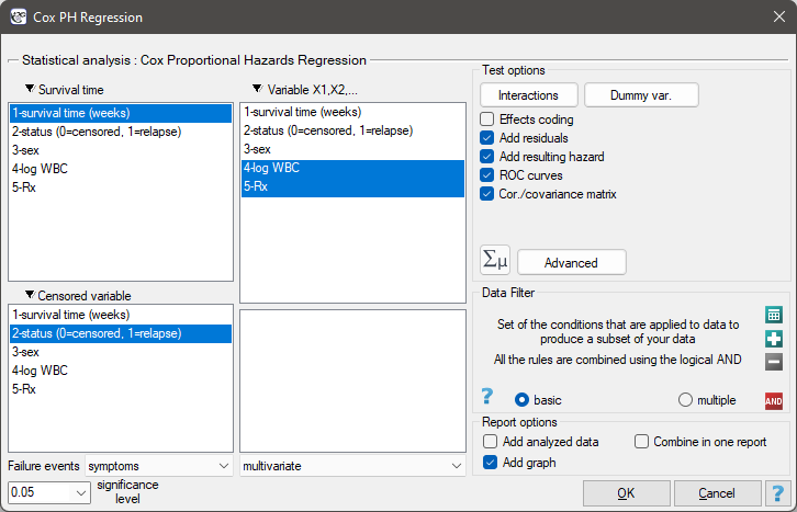
Standard error of a coefficient

\[ SE_b=\sqrt{diag(H^{-1})_b}, \]

where \(diag(H^{-1})\) is the main diagonal of the covariance matrix.

Wald test for a single coefficient
Hypotheses: \(\mathcal{H}_0: \beta_i=0\) against \(\mathcal{H}_1: \beta_i\ne 0\) (equivalently \(\mathcal{H}_0: HR_i=1\) against \(\mathcal{H}_1: HR_i\ne 1\)). Formulas: The test statistic:

\[ \chi^2=\left(\frac{b_i}{SE_{b_i}}\right)^2 \]

asymptotically (for large sample sizes) has the \(\chi^2\) distribution with 1 degree of freedom.

On the basis of the test statistic, the \(p\) value is determined and compared with the significance level \(\alpha\): if \(p \le \alpha\), we reject \(\mathcal{H}_0\) in favor of \(\mathcal{H}_1\); if \(p > \alpha\), there is no reason to reject \(\mathcal{H}_0\).

Information criteria (based on \(L_{FM}\) – the maximum of the likelihood function of the full model, \(L_0\) – the maximum of the likelihood function of the model with the intercept only, \(k\) – the number of parameters, \(d\) – the number of unfavorable events):

\[ AIC=-2\ln L_{FM}+2k,\qquad AICc=AIC+\frac{2k(k+1)}{d-k-1},\qquad BIC=-2\ln L_{FM}+k\ln(d). \]

Pseudo R\(^2\)

\[ R^2_{Pseudo}=1-\frac{\ln L_{FM}}{\ln L_0},\qquad R^2_{Nagelkerke}=\frac{1-e^{-(2/d)(\ln L_{FM}-\ln L_0)}}{1-e^{(2/d)\ln L_0}}, \qquad R^2_{Cox-Snell}=1-e^{\frac{(-2\ln L_0)-(-2\ln L_{FM})}{d}}. \]

Likelihood ratio test for all model variables
Hypotheses: \(\mathcal{H}_0\): all \(\beta_i=0\) against \(\mathcal{H}_1\): there exists \(\beta_i\neq0\). Formulas: The test statistic:

\[ \chi^2=-2\ln(L_0/L_{FM})=-2\ln(L_0)-(-2\ln(L_{FM})) \]

asymptotically (for large sample sizes) has the \(\chi^2\) distribution with \(k\) degrees of freedom.

On the basis of the test statistic, the \(p\) value is determined and compared with \(\alpha\): if \(p \le \alpha\), we reject \(\mathcal{H}_0\) in favor of \(\mathcal{H}_1\); if \(p > \alpha\), there is no reason to reject \(\mathcal{H}_0\).

Time-dependent AUC
For the marker \(M=\sum_{i=1}^k b_iX_i\) and a time \(t\) at which the event of interest occurred, the cumulative/dynamic estimator with IPCW weights (Heagerty et al. 2000[83], Blanche et al. 2013[21]) has the form:

\[ AUC(t)=\frac{\sum_{i}\sum_{j} w_i(t)\,w_j(t)\left[\mathbf{1}(M_i>M_j)+\frac{1}{2}\mathbf{1}(M_i=M_j)\right]}{\sum_i w_i(t)\sum_j w_j(t)}, \]

where the summation over \(i\) covers the cases (\(T_i\le t\), \(\delta_i=1\)) with weight \(w_i(t)=1/\hat G(T_i^-)\), and over \(j\) – the controls (\(T_j>t\)) with weight \(w_j(t)=1/\hat G(t)\); \(\hat G\) is the Kaplan-Meier estimator of the censoring distribution (in which censoring of an observation is treated as the „event”). \(AUC(t)\) is calculated at all unique times of the event of interest, and the mean \(AUC(t)\) given in the report is the arithmetic mean of these values.

Comparison of Cox PH regression models

When to use:

Because of the possibility of simultaneous analysis of many independent variables in one Cox regression model, the problem of choosing the optimal model arises. When selecting independent variables, one should remember that the model should contain variables strongly related to survival time and weakly correlated with one another. Comparing models with different numbers of variables allows us to assess whether adding (or removing) a given variable significantly improves the model.

Definitions of measures

When comparing models we pay attention to the information criteria (\(AIC\), \(AICc\), \(BIC\)) and the model fit coefficients (\(R_{Pseudo}^2\), \(R^2_{Nagelkerke}\), \(R^2_{Cox-Snell}\)), as well as to the result of the likelihood ratio test, which verifies whether the maximum of the likelihood function of the full model (\(L_{FM}\)) differs significantly from that of the reduced model (\(L_{RM}\)).
The decision about the choice of the model is made on the basis of all the above quantities jointly. If the compared models do not differ significantly, we should choose the one with fewer variables – this means that the variables present in the full model and absent in the reduced one do not carry significant information. If the difference is statistically significant, the model with more variables (with the greater \(R^2\)) is significantly better.
In PQStat the comparison of models can be performed in two ways:

manually \(-\) the researcher builds the full model (with more variables) and the reduced one (created from the full model by removing the variables superfluous from the point of view of the studied phenomenon), and then, based on the results of the comparison, chooses the better of them;
automatically \(-\) the program builds successive models itself and indicates the best one according to the chosen criterion (described below).

Automatic model selection
Model terms. The unit that the automatic methods add to or remove from the model is a term: a single variable, a whole dummy variable (all its 0–1 columns at once) or an interaction. The hierarchy principle applies: an interaction can be in the model only when its main effects are in it, and only the interaction can be removed before them.
The selection criterion is chosen in the analysis window:

AIC, AICc or BIC – information criteria; the model with the lower value of the criterion is better. A move (adding or removing a term) is accepted only when it lowers the criterion;
\(p\) of the nested test – the likelihood ratio test comparing the model before and after the change, with a given \(p\) threshold. A term is removed when \(p\) is greater than the threshold, and added when \(p\) is smaller than the threshold. The same \(p\) value is shown in the report as the comparison of neighbouring models;
validation error – the value of \(-2\ln PL\) per event determined out of sample (described below: Out-of-sample evaluation of models). A move is accepted only when it reduces this error. The criterion requires the Validation option to be switched on – choosing it while validation is off switches cross-validation on.

Selection methods:

backward elimination – starts from the model with all the variables; in each step the term whose removal lowers the criterion the most is removed; it ends when no removal lowers the criterion any further;
forward selection – starts from the null model (no variables, the baseline hazard only); in each step the term that lowers the criterion the most is added; it ends when no addition lowers the criterion any further;
bidirectional stepwise – starts from the null model; in each step both additions and removals of terms are considered and the best move is chosen; it ends when no move improves the criterion;
all subsets – all models consistent with the hierarchy principle are fitted (a maximum of 15 terms), and the best model of each size is presented in the report; this method uses the information criteria or the validation error (the \(p\) criterion is not available in it). With many variables the computation may take longer, because the number of fitted models grows exponentially.

All the models are computed on the same set of observations – rows with missing values in any of the candidate variables are discarded once, before the analysis. Thanks to this, the information criteria and the likelihood ratio tests are comparable between models.
The report contains: the selection method and criterion, the number of terms and of fitted models, the information criteria of the null model, the successive models of the selection path (each with the value of \(-2\ln L\), the \(AIC\), \(AICc\) and \(BIC\) criteria, the \(R_{Pseudo}^2\), \(R^2_{Nagelkerke}\) and \(R^2_{Cox-Snell}\) coefficients, and the table of coefficients and hazard ratios) and the comparison of each neighbouring pair of models with the likelihood ratio test (the \(\chi^2\) statistic, degrees of freedom, \(p\) value). The best model according to the chosen criterion is marked in the report. If no term improves the null model, the report states that the null model is the best. With the all subsets method, neighbouring models may not be nested – in that case the test is not performed.

Note! The \(p\) values and confidence intervals in an automatically selected model are too optimistic, because the same data set was used both to select the variables and to estimate their effects. Automatic selection should be treated as an aid in searching for a model, and the final choice should be based on subject-matter knowledge. The selected model should be built again in the Cox PH Regression window and the proportional hazards assumption verified.

Out-of-sample evaluation of models
The information criteria, the fit coefficients and the tests are determined on the same observations on which the coefficients of the models were estimated, which makes the assessment of the models too optimistic – the more so, the more variables the model contains. For this reason, as in comparing multiple regression models, the analysis window makes it possible to evaluate the models on observations that did not take part in fitting them (the Validation option): \(k\)-fold cross-validation (each model is additionally fitted \(k\) times, each time without one of the \(k\) parts of the data) or a random test set (the models are fitted on the training part and evaluated on the test part set aside). The split is random, determined by the Seed, and stratified by status: complete and censored observations are split separately, so that the share of events is similar in every part.
For each model the report then gives two additional measures:

\(-2\ln PL\) per event – the logarithm of the partial likelihood determined out of sample, multiplied by \(-2\) and divided by the number of events. With a test set it is the partial likelihood of the test observations for the coefficients estimated on the training set, and in cross-validation – the cross-validated partial likelihood of Verweij and van Houwelingen[168]. The lower the value, the better the model. This is the validation error – the best model by validation is indicated according to it, and the validation error selection criterion is based on it;
Harrell's C – the concordance index[80]: the percentage of comparable pairs of observations evaluated out of sample in which the observation with the higher predicted risk experienced the event earlier (0.5 – random ordering, 1 – perfect ordering).

The point of reference is the null model (without variables – the same risk for all observations); its validation error is given in the model selection block of the report together with the best model by validation, indicated regardless of the selection criterion chosen. Out-of-sample evaluation also works in the manual comparison of models.

Note! When the validation error is the selection criterion, the validation error of the selected model is slightly too optimistic – out of many models, the one that performed best on the given split was chosen. With a small number of events, the validation results depend on the random split – it is then worth checking them for several values of the seed.

How to set up the analysis

The window with settings for model comparison is accessed via the menu Statistics\(\to\)Survival analysis\(\to\)Cox PH Regression \(-\) comparing models.

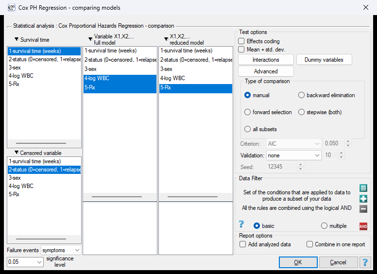
In the window we indicate the survival time, the censored variable with the Failure events value, and the independent variables of the full and the reduced model (in automatic selection – the candidate variables). Model selection options:

Type of comparison – manual or one of the automatic selection methods,
Criterion – AIC, AICc, BIC, p (LR / F test) with the threshold given in the adjacent field, or validation error; in the manual mode the criterion is not used,
Validation – none (evaluation on the training set only), k-fold CV, k = with the number of folds in the adjacent field (from 2 to 100, 10 by default) or test set, % = with the share of the test set as a percentage of the observations (from 5 to 90, 30 by default),
Seed – the seed of the random split of the data (12345 by default); the same seed means the same split.

Calculation and interpretation

Example 2. (remissionLeukemia.pqs file)
The analysis is based on the leukemia data described in the work of Freireich et al. 1963[66] and analyzed further by many authors, including Kleinbaum and Klein 2005[96]. The data contain information about the time (in weeks) of remaining in remission, until the patient was withdrawn from the study because of the end of remission (a relapse of symptoms) or because information about the patient was censored. The end of remission is the unfavorable event – it is treated as a complete observation. An observation is censored if the patient remains in the study to the end and remission does not end, or if the patient leaves the study.
Patients were assigned to two groups: treated traditionally (marked as 1, sometimes called the „placebo group”) and treated with a new method (marked as 0). Information was collected about the patients' sex (1=man, 0=woman) and about the values of the white blood cell count indicator, marked as „log WBC”, which is a known prognostic factor.

The aim of the study is to determine the influence of the treatment method on the time of remaining in remission, taking into account possible confounders and interactions. In the analysis we focus on the „Rx” variable (1=placebo, 0=new treatment); the „log WBC” variable is placed in the model as a possible confounder. To assess the possible effect of the interaction of „Rx” and „log WBC”, we also consider a third variable being their product, added to the model with the Interactions button.

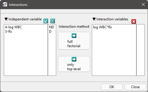
We build three Cox models:

Model A: contains only the „Rx” variable
Model B: contains the „Rx” variable and the potential confounder „log WBC”
Model C: contains the „Rx” variable, the „log WBC” variable and the potential effect of their interaction: „Rx \(\times\) log WBC”

The interaction variable of „Rx” and „log WBC” included in model C is not significant in it (\(p=0.5103\)) according to the Wald test. A similar result is obtained by comparing, with the likelihood ratio test, model C with model B in the Cox PH Regression \(-\) comparing models module: the non-significant result (\(p=0.5134\)) means that model C (with the interaction) is not significantly better than model B (without the interaction).

Comparison of models C and B: \(p=0.5134\) (not significant)

We reject model C – the interaction „Rx” \(\times\) „log WBC” does not contribute significant information. We move on to the comparison of models B and A.

The \(HR\) for „Rx” in model B is 3.65, which means that the hazard for the „placebo group” is about 3.6 times greater than for the group treated with the new method. Model A, containing only the „Rx” variable, is usually called the „crude” model, because it ignores the effect of potential confounders – in this model the \(HR\) for „Rx” is already 4.52, i.e. considerably more than in model B. The 95% confidence interval of these estimators is also important here: for „Rx” in model A its width is 8.06 (10.09 minus 2.03), while in model B it is narrower: 6.74 (8.34 minus 1.60) – so model B gives a more precise estimation of \(HR\) than model A. To finally decide which of them estimates the treatment effect better, we compare them once more with the likelihood ratio test.

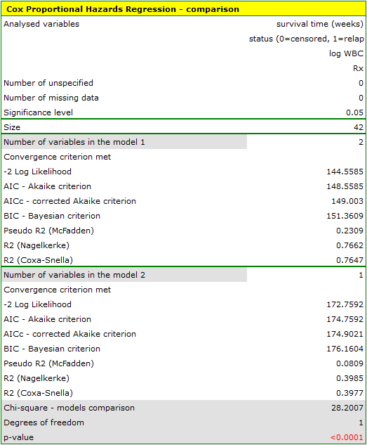
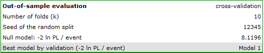
Comparison of models B and A: \(p<0.0001\) (significant)

Model B is significantly better than model A – it has the lowest values of the information criteria (AIC=148.6, AICc=149, BIC=151.4) and high values of fit (Pseudo \(R^2_{McFadden}=0.2309\), \(R^2_{Nagelkerke}=0.7662\), \(R^2_{Cox-Snell}=0.7647\)).

Out-of-sample evaluation. We will also check whether the advantage of model B holds for patients who did not take part in fitting the models. We repeat the comparison of models B and A, choosing in the Validation field the k-fold CV, k = option with 10 folds (seed 12345). In the report model B (full) is marked as Model 1, and model A (reduced) – as Model 2.

	training set	cross-validation (\(k=10\))
model	AIC	\(-2\ln PL\) per event	Harrell's C
null		8.1196
Model B (Rx, log WBC)	148.5585	6.7100	0.8871
Model A (Rx)	174.7592	7.6269	0.7258

Model A, containing only the treatment method, predicts the time of remaining in remission better than the null model (7.6269 versus 8.1196), but it is only the addition of „log WBC” that clearly reduces the validation error (to 6.7100) and raises the concordance of the predictions with the actual order of events from \(C=0.7258\) to \(C=0.8871\). The advantage of model B is therefore not a result of fitting to the data on which it was built – it also holds for patients outside the training set.

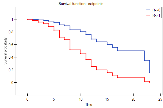
cross-validation (\(k=10\)): \(-2\ln PL\) per event \(=6.71\) (model B), \(7.63\) (model A), \(8.12\) (null model); Harrell's C: \(0.89\) and \(0.73\)

The best model by validation is model B – „log WBC” improves prediction out of sample as well.

The analysis is complemented with the presentation, for model B, of the survival curves (remaining in remission) of both treatment groups, adjusted for the influence of „log WBC”. To plot them, after selecting the Add graph option we check Survival function: in subgroups..., and then – to quickly build a graph of two curves – we choose Quick subgroups and indicate the Rx variable. The Advanced subgroups option allows building any number of arbitrarily defined curves.

Finally, we assess the assumptions of Cox regression by analyzing the model residuals against time.

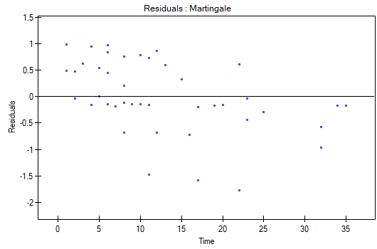
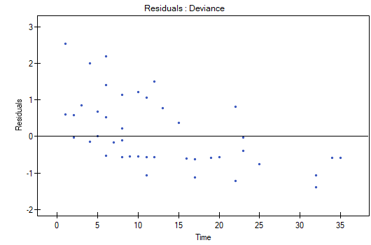
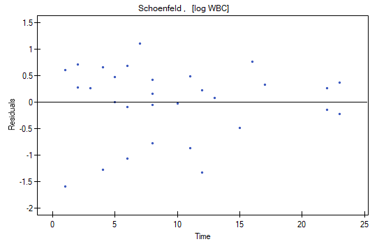
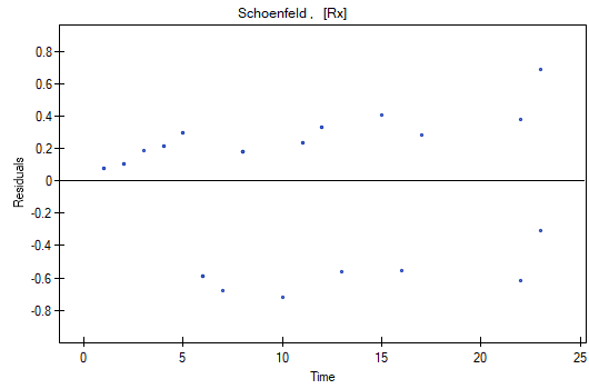
We do not observe outliers, although the Martingale and Deviance residuals become lower for longer times. The Schoenfeld residuals have a symmetrical distribution with respect to time. For the Schoenfeld residuals the analysis of the graph can be supported with tests checking whether the points of the residual plot form some pattern, e.g. a linear relationship – for that purpose we copy the Schoenfeld residuals and time to a datasheet and test the relationship we are looking for. The result of such a test for each variable indicates that the hazard proportionality assumption is fulfilled (when it is not statistically significant) or violated (when it is significant) – such a variable can then be excluded from the model. For the „log WBC” and „Rx” variables the symmetrical distribution of the residuals suggests that the hazard proportionality assumption is fulfilled; this can be confirmed by checking Pearson's linear or Spearman's monotonic correlation of these residuals with time.
Next, we can add the sex variable to the model – with caution, because it is known from the literature that sex may influence the survival function in leukemia remission in a way that is not proportional over time. We therefore build a Cox model for three variables: „Sex”, „Rx” and „log WBC”, and before interpreting the coefficients we check the Schoenfeld residuals – copying them together with time to a new datasheet and checking Spearman's monotonic correlation. We obtain \(p=0.0259\) (for sex), \(p=0.6192\) (for log WBC) and \(p=0.1490\) (for Rx), which confirms the violation of the hazard proportionality assumption by the sex variable.

Schoenfeld residuals vs time: \(p=0.0259\) for sex (significant)

The „Sex” variable violates the hazard proportionality assumption – we build the Cox model separately for women and men, performing the analysis twice with the data filter switched on (first for the female sex, then for the male sex).

For women

For men

FOR THOSE INTERESTED

Out-of-sample evaluation
Let \(\ell(\beta)\) denote the logarithm of the partial likelihood (with the Breslow correction for tied times) determined for the coefficients \(\beta\). Cross-validation uses the cross-validated partial likelihood of Verweij and van Houwelingen[168]:

\[ CVPL=\sum_{j=1}^{k}\left[\ell\left(\hat{\beta}_{(-j)}\right)-\ell_{(-j)}\left(\hat{\beta}_{(-j)}\right)\right], \]

where \(\hat{\beta}_{(-j)}\) are the coefficients estimated without the \(j\)-th part of the data, \(\ell\) – the logarithm of the partial likelihood of all the observations, and \(\ell_{(-j)}\) – of the observations without the \(j\)-th part. The validation error is \(-2\,CVPL/d\), where \(d\) is the number of events. With a test set the validation error is \(-2\,\ell_{T}(\hat{\beta}_{U})/d_T\), where \(\ell_T\) is the logarithm of the partial likelihood of the test observations, \(\hat{\beta}_{U}\) – the coefficients estimated on the training set, and \(d_T\) – the number of events in the test set. In the null model \(\beta=0\) is assumed.

Harrell's C[80] is the ratio of the number of concordant pairs to the number of comparable pairs; the pairs are formed within each evaluated part of the data (in cross-validation – within each fold, for the predictions of the model fitted without that fold) and counted jointly. A pair is comparable when the observation with the shorter time is complete, and concordant – when that observation has the higher predicted risk (a pair with equal predicted risk counts as half of a concordant pair).

Cox regression with time-dependent variables

When to use:

The basic assumption of the Cox model is hazard proportionality: the effect of each independent variable on the hazard must be constant over time, i.e. the Hazard Ratio \(HR_i\) does not change as time passes. When this assumption is violated for one of the variables (an indication may be, e.g., a non-random, systematic pattern of the Schoenfeld residuals against time – see Analysis of model residuals), one of the solutions – besides stratifying the analysis (separate models built for each level of that variable) – is to extend the model with an additional term describing how the effect of the variable changes over time.

Definitions of measures

The extension of the model consists in adding a term being the product of the studied independent variable \(X_j\) and some function of time \(g(t)\):

\[ h(t,X_1,...,X_k)=h_0(t)\cdot\exp\left(\sum_{i=1}^k\beta_iX_i+\delta\cdot X_j\cdot g(t)\right), \]

where the product \(X_j\cdot g(t)\) is called a time-dependent variable (time-dependent covariate). As a result, the partial hazard associated with the variable \(X_j\) is no longer constant and depends on time:

\[ HR_j(t)=e^{\beta_j+\delta\cdot g(t)}. \]

The Wald test for the coefficient \(\delta\) allows checking whether the effect of the variable \(X_j\) really changes over time: \(\delta=0\) means that the effect of \(X_j\) is constant (the hazard proportionality assumption is fulfilled), and \(\delta\ne0\) – that the effect changes over time (the assumption is violated).
In PQStat the function \(g(t)\) can be chosen from among four additional time pseudo-variables, with which a product is built with any independent variable of the model:

time (linear) \(-\) \(g(t)=t\),
ln(time) \(-\) \(g(t)=\ln(t)\),
sqrt(time) \(-\) \(g(t)=\sqrt{t}\),
step(time) \(-\) \(g(t)\) is a step (Heaviside) function, taking the value 0 before a fixed time threshold and 1 after it is exceeded.

How to set up the analysis

The window with settings for Cox regression with time-dependent variables is accessed via the menu Statistics\(\to\)Survival analysis\(\to\)Cox PH Regression – the same window as for standard Cox regression, in which we additionally check the Time-dependent variables option. Once it is checked and the variable defining the survival time is selected, the four additional time pseudo-variables listed above appear on the list of variables used for building interactions (the Interactions button) – so the function \(g(t)\) is defined by choosing one of them.

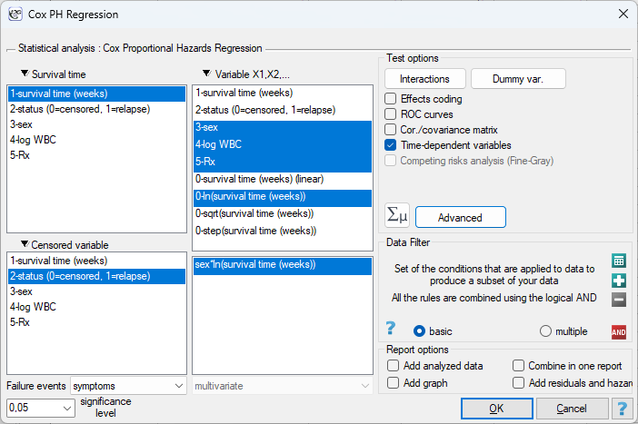
Note! The Time-dependent variables option and the Competing risks analysis (Fine-Gray) option are mutually exclusive.

In the advanced settings window (the gear-icon button), besides the already known convergence parameters of the Newton-Raphson algorithm, two additional parameters related to time-dependent variables are available:

the value \(a\) used to calculate \(\ln(t+a)\) for observations whose survival time equals 0 (by default the logarithmic function is not defined in that case),
the threshold for the step function \(-\) it can be the median of the variable defining time (the default option) or any other value indicated by the researcher.

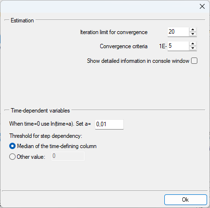
Calculation and interpretation

Example (2) cont. (remissionLeukemia.pqs file)
In the leukemia remission example the analysis of Schoenfeld residuals showed a violation of the hazard proportionality assumption by the sex variable (1=man, 0=woman; a significant monotonic relationship between the residuals and time, p=0.0259), while for the Rx and log WBC variables the assumption was fulfilled. Before we build the extended model, let us look at what this violation looks like in the data and what it leads to in an ordinary Cox model.
Step 1. Kaplan-Meier curves for sex
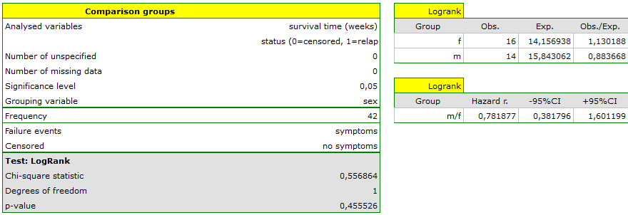
The comparison of the survival curves (remaining in remission) of women and men in the Comparison of groups module gives a non-significant result: log-rank test \(\chi^2=0.56\), \(p=0.4555\), hazard ratio \(HR_{m/f}=0.78\) (95%CI: \(\langle\)0.38; 1.60\(\rangle\)).

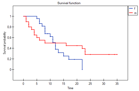
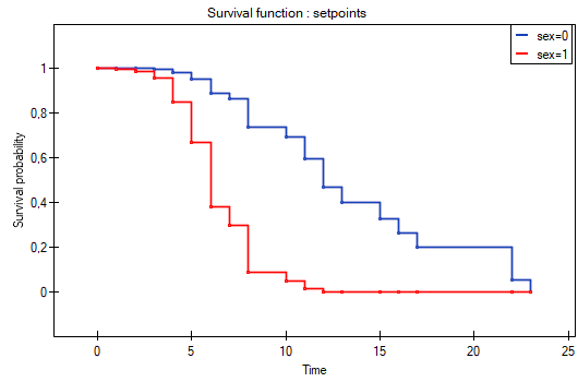
The graph, however, shows why the test „does not see” the difference: the curves cross at about week 11–12. In the first weeks men leave remission much faster (their curve lies lower), but those who get through that period stay in remission longer than women – after week 12 the curve for men lies higher and stabilizes at about 0.28, while the curve for women drops to 0. Crossing curves are the classic picture of a violation of the hazard proportionality assumption: the hazard of men relative to women is not constant but changes direction over time. The log-rank test, which assigns the same weight to all time points, sums differences of opposite signs – and loses power.
Step 2. A Cox model ignoring the violation of the assumption
The same „cancelling out” effect is observed in an ordinary Cox model with three variables: sex, log WBC and Rx.

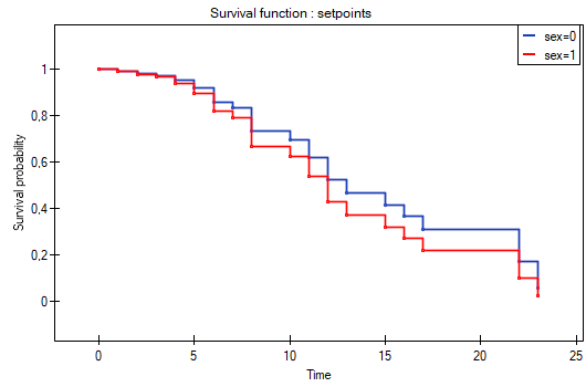
The coefficient of the sex variable is not significant (\(HR=1.30\), 95%CI: \(\langle\)0.54; 3.14\(\rangle\), \(p=0.5582\)), and the survival curves for both sexes plotted from the model (at the means of the other variables) lie close to each other and – by the model's assumption – cannot cross. The model averages the early, very unfavorable effect of being a man with the later favorable effect and ends up with „nothing”. The conclusion that sex is irrelevant to remission time would therefore be wrong – it is an artifact of the unfulfilled assumption.
Step 3. A Cox model with a time-dependent variable
Instead of splitting the analysis into two separate models (for women and for men), we build one joint model in which sex interacts with a function of time. Because we are interested not in whether, but in how, as time passes, the effect of sex changes, we choose the logarithmic function \(g(t)=\ln(t)\) – the effect of clinical variables in survival analysis usually changes fastest at the beginning of follow-up and stabilizes with time, which is well captured by the logarithm. In the analysis window we check the Time-dependent variables option, and in the Interactions window we define the product sex\(\times\)ln(time). The model thus contains four terms: sex, log WBC, Rx and sex\(\times\)ln(time).

The coefficient of the sex\(\times\)ln(time) interaction is \(\delta=-1.912\) (\(SE=0.922\), \(\chi^2_{Wald}=4.30\), \(p=0.0380\)) and is statistically significant – this formally confirms that the effect of sex changes over time, i.e. what the Schoenfeld residuals and the crossing Kaplan-Meier curves suggested earlier. The coefficient of the sex variable itself has also become significant: \(\beta_{sex}=4.057\) (\(p=0.0369\)).
When interpreting these two coefficients, one has to remember that \(\beta_{sex}\) describes the effect of sex only at \(t=1\) (because \(\ln(1)=0\)), and not the effect averaged over the whole follow-up period. The hazard of men relative to women in any week \(t\) is calculated from the formula \(HR_{sex}(t)=e^{\beta_{sex}+\delta\cdot\ln(t)}=e^{4.057-1.912\cdot\ln(t)}\):

\(t\) (weeks)	1	2	4	8	12	16	23
\(HR_{sex}(t)\)	57.8	15.4	4.1	1.1	0.50	0.29	0.14

At the beginning of follow-up the risk of leaving remission is many times higher for men than for women, but this excess decreases quickly; after about 8 weeks (\(t^*=e^{4.057/1.912}\approx 8.4\)) the hazards of both sexes become equal, and later the direction of the relationship reverses – men who have remained in remission now have a risk of relapse several times lower than women. This is exactly the picture shown by the Kaplan-Meier curves in step 1 – the model with a time-dependent variable not only confirms it, but allows it to be measured, with simultaneous adjustment for log WBC and Rx.

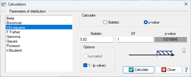
The extended model is also simply better than the model from step 2: it has a higher likelihood (\(-2\ln L=138.4\) versus \(144.2\)), lower information criteria (\(AIC=146.4\) versus \(150.2\); \(BIC=152.0\) versus \(154.4\)) and higher fit coefficients (Pseudo \(R^2_{McFadden}=0.264\) versus \(0.233\)). The likelihood ratio test comparing both models (a difference in \(-2\ln L\) of \(5.82\) with 1 degree of freedom) gives \(p=0.0158\), i.e. adding the time-dependent term significantly improves the model.

\(\delta_{sex\times\ln(t)}=-1.91\), \(p=0.0380\); \(HR_{sex}(t)\) from 57.8 (\(t=1\)) through 1.0 (\(t\approx8.4\)) to 0.14 (\(t=23\))

The effect of sex is not constant over time: men have a much higher risk of leaving remission in the first weeks, and a much lower one later. The ordinary Cox model (and the log-rank test) average these opposite effects into a non-significant „no difference”; the model with a time-dependent variable reveals and measures this change.

FOR THOSE INTERESTED

Wald test for the coefficient of the interaction with the time variable
Hypotheses:

\[\begin{array}{cl} \mathcal{H}_0: & \delta=0 \quad (\text{the effect of } X_j \text{ is constant over time \text{-} the hazard proportionality assumption is fulfilled}),\\ \mathcal{H}_1: & \delta\ne0 \quad (\text{the effect of } X_j \text{ changes over time \text{-} the hazard proportionality assumption is violated}). \end{array}\]

The test statistic and the way of inference are analogous to the Wald test for the other coefficients of the Cox model.

Competing risks analysis – the Fine-Gray model

When to use:

In many studies the observed subjects may experience one of several, mutually exclusive types of unfavorable events. For example, an oncological patient may die because of the underlying disease, but may also die of an entirely different cause (e.g. cardiovascular), before the event of interest occurs. The occurrence of such an alternative event is called a competing risk – it prevents the event of interest from being observed, and at the same time it is not ordinary censoring, because it provides additional information (we know why the observation ended).
Applying the standard Cox model, in which competing events would be treated as ordinary censoring, leads to biased estimates – the standard \(1-S(t)\) function then overestimates the true risk of the event of interest, because some subjects would never have experienced it (they died earlier of a different cause). The appropriate tool for analysis in such a situation is the cumulative incidence function (CIF) together with the Fine-Gray regression model (Fine and Gray 1999)[64], based on the so-called subdistribution hazard.

Definitions of measures

The cumulative incidence function (CIF) expresses, for the event of interest, the probability of its occurrence up to time \(t\), taking into account the fact that competing events may prevent it. The sum of the CIF for the event of interest, the CIF for the competing events and the survival function \(S(t)\) equals 1 at every time point.
The Fine-Gray subdistribution hazard model defines the subdistribution hazard \(h^*(t)\) in a way analogous to how the Cox model describes the standard hazard, but it is based on a different risk set: subjects who experienced the competing event are not removed from the risk set – they remain in it (with an appropriate weight) until the end of follow-up, simulating a situation in which they could never experience the event of interest, but are still being observed. These weights (inverse probability of censoring weighting, IPCW) are calculated from the inverse of the Kaplan-Meier estimator of the censoring distribution. The model parameters are estimated – just like in the standard Cox model – by the maximum likelihood method (the iterative Newton-Raphson algorithm), with the difference that the likelihood function takes into account the IPCW weights described above.
Subdistribution Hazard Ratio (sHR) – for each independent variable a subdistribution hazard ratio (\(sHR\)) is calculated. Unlike the standard \(HR\) of the Cox model (which describes the effect of a variable on the rate of occurrence of the event of interest only among subjects still „at risk” of that event), \(sHR\) describes the effect of the independent variable directly on the cumulative incidence function \(CIF(t)\), which makes it easier to interpret clinically (e.g. for prognosis) in the context of competing risks. The direction of interpretation (\(sHR>1\), \(sHR<1\), \(sHR\approx1\)) is analogous to that of the standard \(HR\) described earlier, and the significance of individual coefficients is likewise verified with the Wald test.

Note! The Fine-Gray model is a separate model from the standard Cox model computed on the same data in which competing events are simply excluded or ignored (treated as no event) – the two models answer different research questions and can lead to different, sometimes even opposite, conclusions (the so-called sign reversal effect described in the literature) for the same independent variable.

How to set up the analysis

The window with settings for the Fine-Gray model is accessed via the menu Statistics\(\to\)Survival analysis\(\to\)Cox PH Regression – the same window as for standard Cox regression, in which we additionally check the Competing risks analysis (Fine-Gray) option. Once it is checked, based on the values of the variable selected as the censoring variable, a Competing event(s): list appears, on which we indicate – among the values other than the code of the event of interest – one or more values denoting competing events. Status values selected neither as the event of interest nor as a competing event remain true censoring.

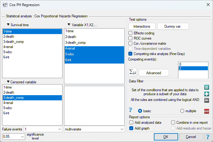
Note! Because model residuals are calculated differently (Martingale, Deviance and Schoenfeld residuals are not defined for the CIF), the Add residuals and hazard option is unavailable for the Fine-Gray model, as is checking the Time-dependent variables option at the same time. The ROC curve option, i.e. the time-dependent AUC, is available – in a version accounting for competing events (see below).

In the report from a Fine-Gray analysis the counts of complete and censored observations are additionally broken down by the code (value of the status variable) they correspond to, and the number of censored observations is further split into the individual competing events. The standard \(HR\) column is replaced with an \(sHR\) (Fine-Gray) column.
Analogously to the standard Cox model (the Add graph option), for the Fine-Gray model the program allows plotting cumulative incidence function (CIF) graphs:

the baseline CIF \(-\) the cumulative incidence at the mean values of the covariates,
CIF for selected variable values \(-\) analogously to the survival function in the standard Cox model, for values of the independent variables indicated by the researcher,
CIF for subgroups \(-\) separate CIF curves built for each category of the indicated grouping variable (the Quick subgroups / Advanced subgroups options).

Note! Unlike the Kaplan-Meier survival function, the CIF curve usually does not tend to 0 or to 1 – its limiting value is the estimated probability that a given subject will ever experience the event of interest before experiencing a competing event.

Time-dependent AUC for competing risks. The ability of the Fine-Gray model to discriminate patients who will experience the event of interest is assessed – as for the standard Cox model – with the time-dependent AUC, with one important difference in the definition of controls. The cases at time \(t\) are only the subjects who experienced the event of interest up to time \(t\); the controls are both the subjects observed longer than \(t\) without any event and the subjects who experienced a competing event up to time \(t\) – they will certainly no longer experience the event of interest, and a good model should assign them a lower risk. The interpretation of \(AUC(t)\) remains unchanged: 0.5 – random discrimination, 1 – perfect discrimination; the graph of \(AUC(t)\) against time (the ROC curve option in the Add graph window) shows how the quality of the prediction of the event of interest changes for successive time horizons.

Calculation and interpretation

Example 3. (multipleMyeloma_competingRisks.pqs file)
In a study of 445 patients diagnosed with multiple myeloma, the efficacy of a new drug (the int variable: 0=standard treatment, 1=new drug) in prolonging survival time (the time variable, in days) was compared. For the patients the baseline white blood cell count (wbc) and the presence of renal failure (renal) were also recorded – a complication frequently accompanying multiple myeloma and considered an unfavorable prognostic factor.

The death of a patient could occur because of the progression of the cancer (the event of interest) or from an entirely different cause, e.g. cardiovascular or infectious, not directly related to the myeloma (the competing event). This information is coded by the death_comp variable: 0 – the patient is alive at the end of follow-up (censoring), 1 – death from myeloma, 2 – death from another cause. The data also contain a simplified death variable (death from any cause, without distinguishing the reason), usually used for the standard Cox model.
The standard model (not appropriate for these data)
For comparison we first build a standard Cox model based on the death variable, in which death from a cause other than myeloma (the competing event) is incorrectly treated the same way as death from myeloma (the event of interest):

The Fine-Gray model
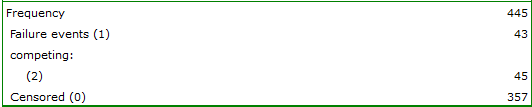
Next we build the model appropriate for these data – the Fine-Gray model – indicating death_comp as the censoring variable, code 1 (death from myeloma) as the event of interest, and checking code 2 (death from another cause) on the Competing event(s): list.

The obtained \(sHR\) for the int variable is \(sHR=0.67\) (95%CI: \(\langle\)0.25; 1.80\(\rangle\)), \(p=0.4235\), which means there is no basis to claim that the new drug significantly affects the risk of death from multiple myeloma once the competing risk of death from another cause is properly accounted for. A different picture is given by the standard model (incorrectly ignoring the distinction between causes of death), in which the \(HR\) for int is \(HR=2.18\), \(p=0.008034\) – suggesting a significant, unfavorable effect of the new drug on the risk of death from any cause. This is a good illustration of the sign reversal effect described earlier: the drug may slightly increase the risk of death from other causes (e.g. as a result of adverse effects), which in the standard model is mixed with the risk of death from the cancer itself, suggesting an apparent unfavorable effect of the drug on the course of the myeloma – while the Fine-Gray model shows that the drug has no significant effect on the risk of death specifically from myeloma.

\(HR_{int}=2.18\), \(p=0.008034\) (standard model) versus \(sHR_{int}=0.67\), \(p=0.4235\) (Fine-Gray model)

The new drug apparently increases the overall risk of death, but does not significantly increase the risk of death specifically from myeloma – the effect visible in the standard model disappears once competing events are properly accounted for.

The opposite situation is observed for renal failure (renal) – here both models consistently indicate a strong, statistically significant relationship with the risk of death, and in the Fine-Gray model the effect is even more pronounced: \(sHR=38.65\) (95%CI: \(\langle\)19.47; 76.72\(\rangle\)), \(p<0.000001\), versus \(HR=11.39\) (95%CI: \(\langle\)7.08; 18.32\(\rangle\)), \(p<0.000001\) in the standard model. Renal failure is therefore not only a significant risk factor for death from any cause, but above all strongly – and even more strongly than the standard model would suggest – related to the risk of death from the progression of the myeloma itself, which is consistent with its well-known role as an unfavorable prognostic factor in this disease (kidney damage usually accompanies an advanced form of myeloma).

\(sHR_{renal}=38.65\), 95%CI: \(\langle\)19.47; 76.72\(\rangle\), \(p<0.000001\) (Fine-Gray model) versus \(HR_{renal}=11.39\), \(p<0.000001\) (standard model)

Renal failure is strongly and consistently related to the risk of death from myeloma – the effect is even more pronounced once the competing risk of death from another cause is properly accounted for.

Finally, we compare the CIF curves for death from myeloma in the groups defined by the renal variable:

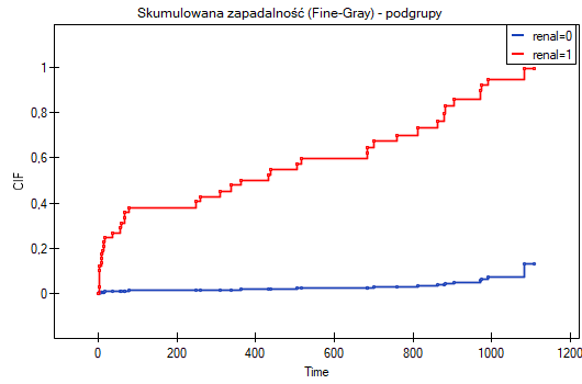
The CIF curve for patients with renal failure (renal=1) rises much faster and reaches much higher values than the curve for patients without this complication (renal=0) – already after about 100 days of follow-up the cumulative probability of death from myeloma in this group exceeds 0.4, and towards the end of follow-up it approaches 1. In patients without renal failure the cumulative probability of death from myeloma remains low (below 0.15) throughout the follow-up period. The graph thus confirms the numerical \(sHR\) result: in these data renal failure is associated with a significantly higher risk of death from multiple myeloma.
Finally, we assess the ability of the built Fine-Gray model to discriminate the patients who will die from myeloma, by selecting the ROC curve option in the Add graph window, i.e. the graph of the time-dependent AUC:

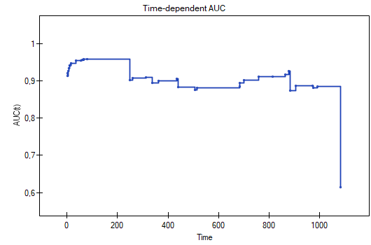
The values of \(AUC(t)\) are high throughout the follow-up period. In the first weeks \(AUC(t)\) rises from about 0.91 to about 0.96 and stays at this level for the first approx. 250 days, and then – as the controls lose event-free patients and gain deaths from other causes – it decreases to the level of 0.88–0.92, at which it remains almost until the end of follow-up. This means that the model (and in practice mainly the renal variable) discriminates very well between patients who will die from myeloma by a given time \(t\) and those who will not die from this cause by that time – regardless of the prediction horizon. The sharp drop of \(AUC(t)\) at the last point (about 1080 days) is an estimation artifact: at such a late time only a few observations remain in the risk set, and an estimator based on a handful of case–control pairs becomes unstable; the values at the very end of the time axis should therefore not be interpreted.

\(AUC(t)\approx 0.88\)–\(0.96\) for \(t\) from a few to about 1000 days

The Fine-Gray model discriminates patients at risk of death from myeloma very well and stably over time – the quality of the prediction does not depend significantly on the adopted time horizon.

FOR THOSE INTERESTED

Cumulative incidence function (CIF)

\[ CIF(t)=P(T\le t,\ \varepsilon=1)=\sum_{t_i\le t}S(t_{i-1})\cdot h_1(t_i), \]

where \(S(t_{i-1})\) is the overall (all-cause) survival function just before \(t_i\), and \(h_1(t_i)\) is the cause-specific hazard for the event of interest at \(t_i\).

The Fine-Gray subdistribution hazard model

\[ h^*(t,X_1,...,X_k)=h^*_0(t)\cdot\exp\left(\sum_{i=1}^k\beta_iX_i\right) \]

The IPCW weights used to keep subjects in the risk set after the occurrence of a competing event are calculated from the inverse of the Kaplan-Meier estimator of the censoring distribution \(\hat G(t)\):

\[ w_i(t)=\frac{\hat G(t)}{\hat G(\min(T_i,t))}, \]

where the estimator \(\hat G\) is calculated the same way as the Kaplan-Meier estimator of the survival function, but with the roles reversed – true censoring is treated here as the „event”, while both the event of interest and the competing events are treated as censoring for this auxiliary estimator.

Subdistribution Hazard Ratio (sHR)

\[ sHR_i=e^{\beta_i}. \]

Time-dependent AUC for competing risks
The formula is the same as for the standard Cox model (see Cox proportional hazards regression); only the set of controls and their weights change: besides the subjects with \(T_j>t\) (weight \(1/\hat G(t)\)), the controls also include the subjects who experienced a competing event up to time \(t\) (\(T_j\le t\), \(\varepsilon_j=2\)), with weight \(1/\hat G(T_j^-)\). The estimator \(\hat G\) is the same Kaplan-Meier estimator of the censoring distribution that is used to determine the IPCW weights of the model (Blanche et al. 2013[21]).