The Durbin's ANOVA (missing data)

When to use this test:

Durbin's analysis of variance of repeated measurements for ranks (Durbin, 1951[54]) is used in the same situation as the Friedman ANOVA – when measurements of the analysed variable are taken several times on the same objects. The Durbin test has an advantage, though: it can also be calculated for an incomplete data set, provided the missing values form a so-called balanced and incomplete block (each object has the same number of measurements, and each pair of measurements occurs together equally often).

Assumptions

measurement on an ordinal scale or an interval scale,
a dependent model,
if present, missing data form a balanced and incomplete block: each object has the same number \(k\) of measurements, each measurement concerns the same number \(r\) of objects, and the number of objects for which the same pair of measurements was taken simultaneously is constant.

How to set up the analysis

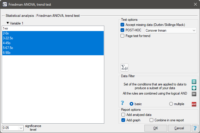
Statistics \(\to\) Nonparametric tests \(\to\) Friedman ANOVA (missing data allowed).

Step 1. Select the variables corresponding to successive measurements.

Step 2. Select the Accept missing data option if the data contain gaps.

Step 3. If the test shows a significant difference, select the Conover-Inman POST-HOC test.

Step 4. Run the analysis.

Note! For records with missing data to be taken into account, the Accept missing data option must be selected. Empty cells and cells with non-numeric values are treated as missing data. Only records containing more than one numeric value are included in the analysis.

Performing and interpreting the analysis

Example 1. (mirror.pqs file)
An experiment was conducted among 20 patients in a psychiatric hospital (Ogilvie, 1965[130]), involving drawing straight lines according to a presented pattern – 5 lines drawn at different angles (\(0^o\), \(22.5^o\), \(45^o\), \(67.5^o\), \(90^o\)) relative to the indicated center. The patients' task was to reproduce the lines with their hand covered, and the outcome was the time it took to draw each line. Because of fatigue and limited patient cooperation, the project was planned in a balanced and incomplete block: each of the 20 patients drew a line at two of the five possible angles, so that each angle was drawn eight times in total. We want to check whether the time spent drawing each line is entirely random, or whether some lines took more or less time to draw. The time (in seconds) each patient took to draw the line at a given angle was recorded in the table.

patient number	\(0^o\)	\(22.5^o\)	\(45^o\)	\(67.5^o\)	\(90^o\)
1	7	15
2	20		72
3	8			26
4	33				36
5	7	16
6		68	67
7		33		64
8		34			12
9	10		96
10		29	59
11			17	9
12			100		15
13	16			32
14		19		32
15			36	39
16				44	54
17	16				38
18		17			12
19			37		11
20				56	6

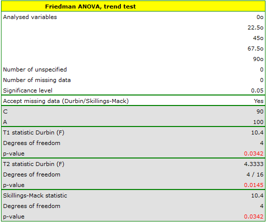
\(p=0.014541\) for the \(T_2\) statistic (or \(p=0.034203\) for \(T_1\)), statistically significant, \(\alpha=0.05\)

The time spent drawing each line is not the same.

The POST-HOC analysis performed indicates a difference in the time spent drawing the line at angle \(0^o\) – it is drawn faster than the lines at \(22.5^o\), \(45^o\) and \(67.5^o\).

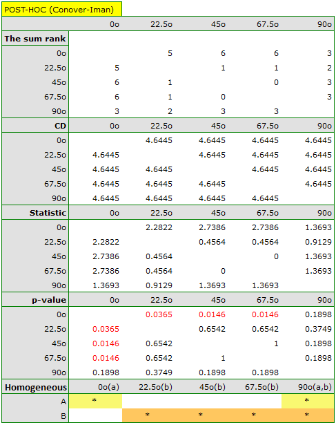
The graph shows the homogeneous groups indicated by the POST-HOC test.

FOR THOSE INTERESTED

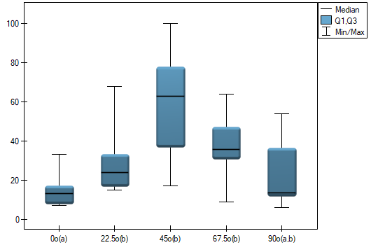
Hypotheses: they relate to the equality of the sum of ranks for successive measurements (\(R_j\)) or are simplified to medians (\(\theta_j\)):

\[\begin{array}{cl} \mathcal{H}_0: & \theta_1=\theta_2=...=\theta_t,\\ \mathcal{H}_1: & \text{not all }\theta_j\text{ are equal }(j=1,2,...,t), \end{array}\]

where \(t\) – total number of measurements considered, \(b\) – total number of objects studied.

Formulas: two test statistics are determined:

\[ T_1=\frac{(t-1)\left[\sum_{j=1}^tR_j^2-tC\right]}{A-C}, \]

\[ T_2=\frac{T_1/(t-1)}{(b(k-1)-T_1)/(bk-b-t+1)}, \]

where:
\(R_{j}\) – sum of ranks for successive measurements \((j=1,2,...t)\),
\(R_{ij}\) – ranks assigned to successive measurements, separately for each object studied \((i=1,2,...b)\),
\(\displaystyle A=\sum_{i=1}^b\sum_{j=1}^tR_{ij}^2\) – sum of squared ranks,
\(\displaystyle C=\frac{bk(k+1)^2}{4}\) – correction coefficient. The formula for \(T_1\) and \(T_2\) includes a correction for tied ranks.

For complete data, the \(T_1\) statistic is identical to the Friedman test and asymptotically (for large sample sizes) has the \(\chi^2\) distribution with \(df=t-1\) degrees of freedom. The \(T_2\) statistic is the equivalent of the Iman-Davenport correction of the Friedman ANOVA, and follows the F Snedecor distribution with \(df_1=t-1\) and \(df_2=bk-b-t+1\) degrees of freedom – it is now considered more precise than the \(T_1\) statistic and is recommended for use[48].

The \(p\) value, determined on the basis of the test statistic, is compared with \(\alpha\): if \(p \le \alpha\), we reject \(\mathcal{H}_0\) in favor of \(\mathcal{H}_1\); if \(p > \alpha\), there is no reason to reject \(\mathcal{H}_0\).

POST-HOC tests

An introduction to contrasts and POST-HOC tests is provided in section Contrasts and POST-HOC tests, which concerns the one-way analysis of variance.

The Conover-Inman test
Used for simple comparisons (the counts in each measurement are always the same).

\(\mathfrak{(i)}\)
The critical difference is calculated using the formula:

\[ CD=t_{1-\alpha /2, bk-b-t+1}\sqrt{\frac{(A-C)2r}{bk-b-t+1}\left(1-\frac{T_1}{b(k-1)}\right)}, \]

where \(t_{1-\alpha /2, bk-b-t+1}\) is the critical value (statistic) of the \(t\)-Student distribution for the significance level \(\alpha\) and \(df=bk-b-t+1\) degrees of freedom.
\(\mathfrak{(ii)}\)
The test statistic is defined by:

\[ t=\frac{\sum_{j=1}^k c_jR_j}{\sqrt{\frac{(A-C)2r}{bk-b-t+1}\left(1-\frac{T_1}{b(k-1)}\right)}}. \]

The test statistic has the \(t\)-Student distribution with \(df=bk-b-t+1\) degrees of freedom.