 PQStat
RANDOMNESS OF POINT DISTRIBUTION
To conduct analysis of the randomness of point distribution on the basis of a Map data we should have at our disposal a point, multipoint, or polygonal file. In the case of an analysis of a polygonal file, calculations are based on centroids of polygons, and in the case of a multipoint file they are based on centers of objects.
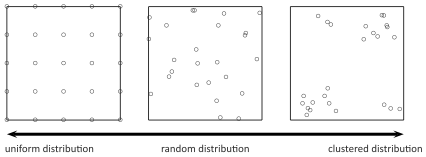
The effect of uniform dispersion appears when points are distributed more regularly than the possible result of random distribution. If the spatial distribution is as probable as any other distribution we speak about spatial randomness. When the points come in groups we speak about clustered distribution.
Nearest Neighbor Analysis
In the Nearest Neighbor Analysis the boundaries of the area in which the analysed points are enclosed have the crucial influence on the result. The example below illustrates regularly distributed points and their clustered distribution when bounded by a large rectangle.

Depending on the needs, the bounding can be defined with the help of: a convex hull, the smallest rectangle, a rectangle from layer bounding, or the smallest circle. The studied area can also be defined only with the use of the size of its area.
The distance between the points is measured with the Euclidean metric.
The first stage of the nearest neighbor analysis is calculating the distance among all points. Next, for each point we search for the nearest point, i.e. for the nearest neighbor (\(NN\)).
Note
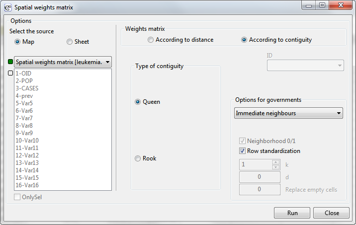
The distances between all points are defined by a spatial weight matrix. In Moran's analysis window we can choose matrix generated previously by using menu Spatial analysis \(\to\) Tools \(\to\) Spatial weights matrix or indicate the neighbor matrix according to contiguity – Queen, row standardized, that is proposed by the program.
The basic statistics for the analysis of the nearest neighbors are:
- \(d_i(NN)\) –the distance of each point from its nearest neighbor,
\(\overline{NN}\) –the mean nearest neighbor distance:
\[ \overline{NN}=\sum_{i=1}^n\frac{d_i(NN)}{n} \]- \(SD_{(NN)}\) –standard deviation of the nearest neighbors distance,
\(\overline{ran}\) –mean random nearest neighbor distance:
\[ \overline{ran}=\frac{0.5}{\sqrt{\frac{n}{A}}} \]
- Nearest Neighbor Index
Nearest Neighbor Index ( NNI) is based on a method described by botanists: Clark and Evans (1954) [4]. \(NNI\) compares distances observed between the nearest points, and distances which would appear for a random distribution of points.\[ NNI=\frac{\overline{NN}}{\overline{ran}} \]When the compared distances are the same then \(NNI=1\). When the observed distances between the nearest points are smaller than expected then the points are nearer to one another than in a random distribution, and \(NNI<1\). In such a case, clusters occur. When the situation is reverse, then \(NNI>1\), which points to the occurrence of the effect of uniform distribution, i.e. points are distributed more regularly than in a case of random distribution.
- Significance of the Nearest Neighbor Index
The test for checking the significance of the Nearest Neighbor Index \(NNI\) serves the purpose of verifying the hypothesis that the distances observed between the nearest points are the same as the expected distances which would appear in a random distribution of points.
Hypotheses:\(\begin{array}{cl} \mathcal{H}_0: & NNI = 1, \\ \mathcal{H}_1: & NNI \ne 1. \end{array}\)
The test statistic has the form presented below:
\[ Z=\frac{\overline{NN}-\overline{ran}}{SE_{\overline{ran}}}, \]where:
\(\begin{array}{cl} SE_{(ran)} = \sqrt{\frac{4-\pi A}{4\pi n^2}} & \textrm{\textendash standard error of the mean random}\\ &\textrm{nearest neighbor distance } \end{array}\)
Statistics \(Z\) asymptotically (for a large sample size) has the normal distribution.
Value \(p\), defined on the basis of test statistics, is compared with the significance level \(\alpha\) :\[ \begin{array}{ccl} \text{ if } p \le \alpha & \Longrightarrow & \text{ we reject } \mathcal{H}_0 \text{ and accept } \mathcal{H}_1, \\ \text{ if } p > \alpha & \Longrightarrow & \text{ there is no reason to reject } \mathcal{H}_0. \\ \end{array}\]- Analysis of Subsequent Nearest Neighbors
To analyse subsequent nearest neighbors one takes into account the distance to the second nearest neighbor, the third nearest neighbor, and so on, to the \(k\)-order nearest neighbor. For the neighborhood of each order (from the nearest neighbor to the \(k\)-order neighbor) subsequent Nearest Neighbor Indexes \(k_{ordered}NNI\) are calculated:\[ k_{ordered}NNI=\frac{k_{ordered}\overline{NN}}{k_{ordered}\overline{ran}} \]where:
\(\displaystyle k_{ordered}\overline{NN}\) –mean distance from neighbors of \(k\)-order,
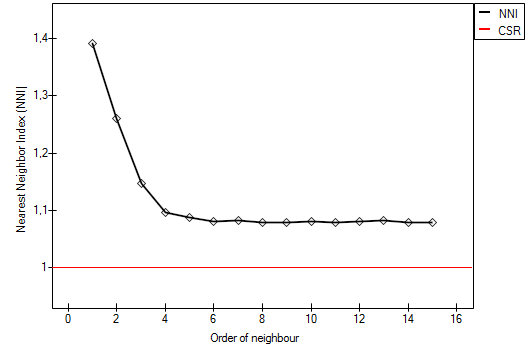
\(\displaystyle k_{ordered}\overline{ran}=\frac{k(2k)!}{\left(2^kk!\right)^2\sqrt{\frac{n}{A}}}\) –mean random distance from neighbors of \(k\)-order.The results of the point density analysis conducted for subsequent neighbors can be presented on a graph so as to illustrate the placement of \(NNI\) in reference to the line which shows the random point structure and so as to check if a growing or falling trend has been achieved for the indexes.
- Edge Effect
Objects placed near the bounding show a tendency to be further away from their nearest neighbors than other objects within the analysed area. The reason for it is the simple fact that the nearest neighbors of the objects near the border can be objects outside the studied area. In such a situation we can conduct an analysis with an adjustment for the edge effect.In such a case the distance of a point from its nearest neighbor (\(d_i(NN)\)) is calculated as the minimum distance of the point from its neighbors and from the boundary. Thus, if the distance of the point from the boundary will be smaller than the distance from its neighbors, then the distance from the boundary is considered to be \(d_i(NN)\). However, such a calculation of the nearest neighbor requires an assumption that there will always be a neighboring point on the border.
The window with settings for Nearest Neighbor Analysis is accessed via the menu Spacial analysis \(\to\) Spatial Statistics \(\to\) Nearest Neighbor Analysis.
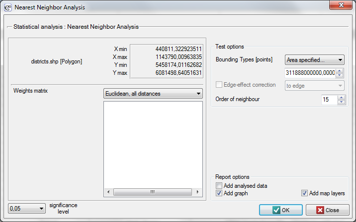
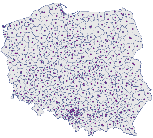
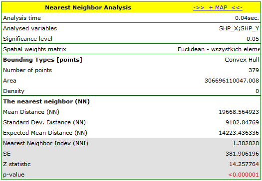
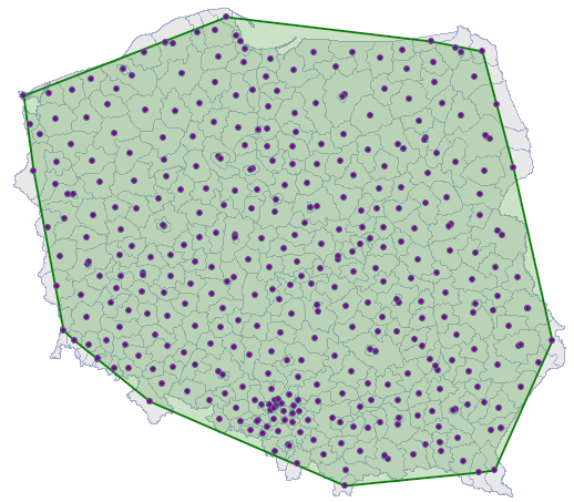
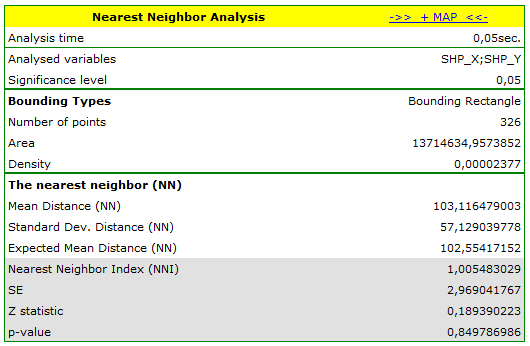
Example 1. (directory: districts, SHP files: districts) The admistrative division of Poland into powiats should, by definition, be uniform. With the use of NNI we will check if that is the case.
The nearest neighbor analysis will be based on centroids representing powiats. We can draw them (add the centroid layer to the map of powiats) with the use of the Map manager.
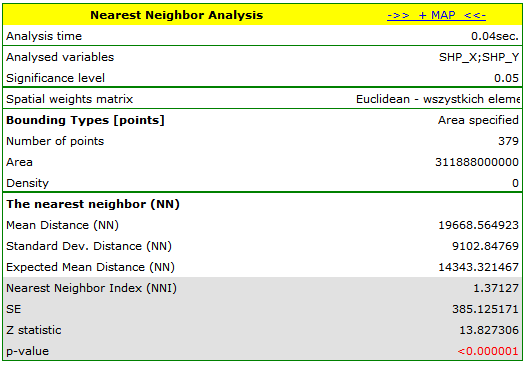
 ) and choose the convex hull as the bounding (\(NNI=1.382828\), \(p<0.000001\)).
 and choosing the layer of bounding.
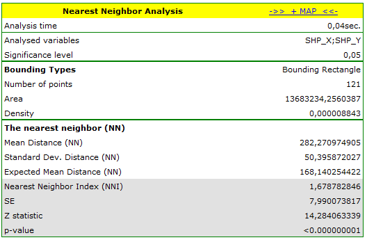
Example 2. (directory: poplar, SHP files: T-poplar, S-poplar) Competition among species has an influence on the changes in the distribution of particular species of plants and on their density. Competition within a species is usually stronger than that among different species as members of the same species have almost identical demands and compete for the same resources. The intensity of competition within a species increases with the growth of the population. To check the influence of the competition on a certain species of balsamic poplar, a wooded area not regulated by man was studied. Locations of young trees and of old ones were studied.
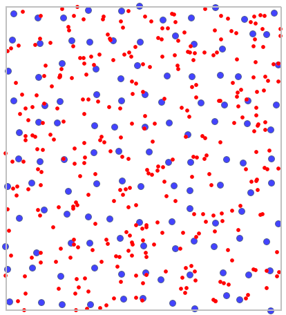
On the basis of the nearest neighbor indices, the structure of poplar density was compared in the area defined by a rectangle of layer bounding.
SPATIAL AUTOCORRELATION
To conduct spatial autocorrelation on the basis of a Map data we should have at our disposal a point, multipoint, or polygonal file. In the case of an analysis of a polygonal file based on the calculation of objects distances, calculations are based on centroids of polygons, and in the case of a multipoint file they are based on centers of objects.
An analysis of the phenomenon of autocorrelation is based on values assigned to spatial objects. Spatial autocorrelation means that the values of geographically near objects are more similar to one another than those of remote objects. The phenomenon causes the creation of spatial clusters with similar values.
Spatial autocorrelation may not occur – we then speak of spatial randomness. The obtained spatial distribution is as probable as any other distribution. When the neighboring values are similar to one another we can speak about positive autocorrelation. Negative autocorrelation occurs when the values of neighboring areas are more varied than in the case of random distribution.
| i | i | i | i | i | i | i | i |
| i | i | i | i | i | i | i | i |
| i | i | i | i | i | i | i | i |
| i | i | i | i | i | i | i | i |
| i | i | i | i | i | i | i | i |
| i | i | i | i | i | i | i | i |
| i | i | i | i | i | i | i | i |
| i | i | i | i | i | i | i | i |
| i | i | i | i | i | i | i | i |
| i | i | i | i | i | i | i | i |
| i | i | i | i | i | i | i | i |
| i | i | i | i | i | i | i | i |
| i | i | i | i | i | i | i | i |
| i | i | i | i | i | i | i | i |
| i | i | i | i | i | i | i | i |
| i | i | i | i | i | i | i |
| i | i | i | i | i | i | i | i |
| i | i | i | i | i | i | i | i |
| i | i | i | i | i | i | i | i |
| i | i | i | i | i | i | i | i |
| i | i | i | i | i | i | i | i |
| i | i | i | i | i | i | i | i |
| i | i | i | i | i | i | i | i |
| i | i | i | i | i | i | i | i |

When analyzing autocorrelation we can consider a dichotomous variable (i.e. the presence or absence of a given feature) or a variable with many categories, pointing to the degree of intensity of the analyzed feature.
For a dichotomous variable the analysis of positive autocorrelation consists of searching for clusters with the same value. Usually, objects in which the studied phenomenon occurs are marked in black color on the map, and the ones in which the phenomenon does not occur are marked in white color. Clusters of objects of the same color – the so-called "black-black","white-white" – are looked for.
For a variable which describes the degree of intensity of a studied feature the analysis of positive autocorrelation consists of searching for clusters with similar values. Usually, objects on the map are colored in accordance with the degree of intensity of the studied phenomenon, from the lightest (low values) to the darkest (high values). Clusters of objects with a similar shade are looked for.
Global Moran's I statistic
It is an analysis of the degree of intensity of a given feature in spatial objects.
We use two pieces of information for the construction of a coefficient which will allow to check if the neighboring objects form clusters with similar values of the variable:
- information about the values of a variable for particular objects \(x_i\),
- information about which objects are neighbors – weights matrix with elements \(w_{ij}\).
Note
The objects neighborhood is defined by a spatial weight matrix. In Moran's analysis window we can choose any matrix generated previously by using menu Spatial analysis \(\to\) Tools \(\to\) Spatial weights matrix or indicate the neighbor matrix according to contiguity – Queen, row standardized, that is proposed by the program.
Note
It is not recommended to conduct Moran's analysis for objects without neighborhood (objects described in the weight matrix only with the 0 value). Such objects can be excluded from the analysis by deactivating them or an analysis can be made with the use of a different manner of defining neighborhood (a different weight matrix).
- Moran's I coefficient
– introduced by Moran in 1948 [9].
In order to check if the selected objects are characterized by similar values of the variable one can use the multiplying rule which says that multiplying 2 positive numbers gives a positive result and multiplying 2 different numbers (1 positive and 1 negative) gives a negative result. With the use of this rule we calculate \(\sum\sum x_ix_j\). Unfortunately, as the results of that rule are only obtained when there are both positive and negative values, the simple rule must be modified so as to ensure the presence of different signs. The values of the variable will, then, be replaced in the earlier formula with the differences of the values of the variable and of its mean value. In this way the objects with values smaller than the mean will be negative and those with values greater than the mean will be positive: \(\sum\sum(x_i-\overline{x})(x_j-\overline{x})\). Obviously, the summation should concern neighboring objects, which means that, at this point, information from weights matrices must be used:\[ \sum\sum w_{ij}(x_i-\overline{x})(x_j-\overline{x}) \]In this way non-neighboring objects obtain the weight value 0, for which reason the values of those objects are not added. Further operations which change the formula obtained in this manner are made with the view to making the obtained coefficient \(I\) independent from the number of analyzed objects and to standardizing it so that its values are limited to the interval \(<-1; 1>\). As a result, Moran's autocorrelation coefficient is expressed with the formula:
\[ I=\frac{\sum_{i=1}^n\sum_{j=1}^nw_{ij}\left(x_i-\overline{x}\right)\left(x_j-\overline{x}\right)}{S_0\sigma^2} \]where:
\(n\) – the number of spatial objects (the number of points or polygons),
\(x_i\), \(x_j\) – are the values of the variable for the compared objects,
\(\overline{x}\) – it is the mean value of the variable for all objects,
\(w_{ij}\) – elements of the spatial weights matrix (weights matrix row standardized),
\(S_0=\sum_{i=1}^n\sum_{j=1}^nw_{ij}\),
\(\sigma^2=\frac{\sum_{i=1}^n\left(x_i-\overline{x}\right)^2}{n}\) – varianceMoran's linear autocorrelation coefficient \(I\) studies the strength of the linear relationship between the standardized variable \(X\) (\(stand(x_i)\)) and the spatial lag of the variable \(X\) (\(L(x_i)\)). Spatial lag is the weighted mean from the standardized values of neighboring objects
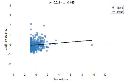
\[ L(x_i)=\sum_{j=1}^Nw_{ij}stand(x_j). \]A graphic presentation of spatial autocorrelation is Moran's scatter plot. Points in the first quarter (HH) and in the third quarter (LL) are objects surrounded by similar neighbors: HH (high-high) – objects with high values, surrounded by objects with high values; LL (low-low) – objects with low values, surrounded by objects with low values. Points in the second quarter (LH) and the fourth quarter (HL) are objects surrounded by neighbors not similar to them. LH (low-high) – objects with low values, surrounded by objects with high values; HL (high-low) – objects with high values, surrounded by objects with low values.
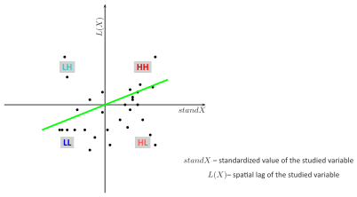 Moran's diagram
The belonging to and distribution of points in the four quarters of Moran's diagram indicates the type of autocorrelation. If points are distributed mainly in the second quarter (LH) and fourth (HL) – it is a sign of negative correlation, if they belong mainly to the first quarter (HH) and third (LL) – it is a sign of positive correlation. If the points are distributed evenly in all four quarters then spatial autocorrelation does not exist.
On the Moran's diagram there is a regression line, the direction of which also allows to interpret Moran's coefficient \(I\):- \(I>0\) indicates the presence of clusters of similar values – positive autocorrelation, i.e. measurement points lie near the straight line, and the increase of the variable \(standX\) is reflected in the increase of the variable \(L(X)\);
- \(I<0\) indicates the presence of the so-called hot spots, i.e. decidedly different values in neighboring areas – negative autocorrelation, i.e. measurement points lie near the straight line but the increase of the variable \(standX\) is accompanied by a decrease of the variable \(L(X)\);
- \(I \approx 0\) indicates random distribution of the studied value in space – a lack of autocorrelation, i.e. the obtained spatial distribution is as probable as any other distribution.
The square of Moran's coefficient \(I^2\) informs about the degree (it is a percentage) to which the value of the variable in the object \(i\) is explained by the value of that variable in neighboring objects.
Note
When the values of a studied feature are characterized by a great variability of variance then it is desirable to stabilize that variability. The basic information about smoothing variables have been described in the Chapter SPATIAL SMOOTHING SPATIAL SMOOTHING- Significance of Moran's autocorrelation coefficient
A test for checking the significance of Moran's autocorrelation coefficient serves the purpose of verifying the hypothesis about a lack of correlation between \(standX\) and spatial lag \(L(X)\).
Hypotheses:\(\begin{array}{cl} \mathcal{H}_0: & I = 0, \\ \mathcal{H}_1: & I \ne 0. \end{array}\)
The test statistic has the form presented below:
\[ Z=\frac{I-E(I)}{\sqrt{var(I)}}, \]where:
\(\displaystyle E(I)=\frac{-1}{n-1}\) – the expected value,
\(\displaystyle var(I)\) – variance.
Depending on the assumption concerning the distribution of the population from which the sample has been taken, the manner of selecting variance is chosen (Cliff and Ord (1981)[5], and Goodchild (1986)[8]). If it is normal distribution, then:\[ var(I)=\frac{n^2S_1-nS_2+3S_0^2}{S_0^2(n^2-1)}-E(I)^2, \]where:
\(S_1=\frac{1}{2}\sum_{i=1}^n\sum_{j=1}^n\left(w_{ij}+w_{ji}\right)^2\),
\(S_2=\sum_{i=1}^n\left(\sum_{j=1}^nw_{ij}+\sum_{j=1}^nw_{ji}\right)^2\).If it is random distribution, then:
\[ var(I)=\frac{n\left((n^2-3n+3)S_1-nS_2+3S_0^2\right)}{(n-1)^{(3)}S_0^2}-\frac{K_2\left((n^2-n)S_1-2nS_2+6S_0^2\right)}{(n-1)^{(3)}S_0^2}-E(I)^2, \]where:
\(K_2=\frac{n\sum_{i=1}^n\left(x_i-\overline{x}\right)^4}{\left(\sum_{i=1}^n\left(x_i-\overline{x}\right)^2\right)^2}\),
\(n^{(b)}=n(n-1)(n-2)...(n-b+1)\).Statistics asymptotically (for a large sample size) has the normal distribution.
On the basis of test statistics, \(p\) value is estimated and then compared with the significance level \(\alpha\) :\[ \begin{array}{ccl} \text{ if } p \le \alpha & \Longrightarrow & \text{ we reject } \mathcal{H}_0 \text{ and accept } \mathcal{H}_1, \\ \text{ if } p > \alpha & \Longrightarrow & \text{ there is no reason to reject } \mathcal{H}_0. \\ \end{array}\]
The window with settings for Moran's analysis is accessed via the menu Spacial statistics\(\to\)Tools\(\to\)Moran's global I statistic.
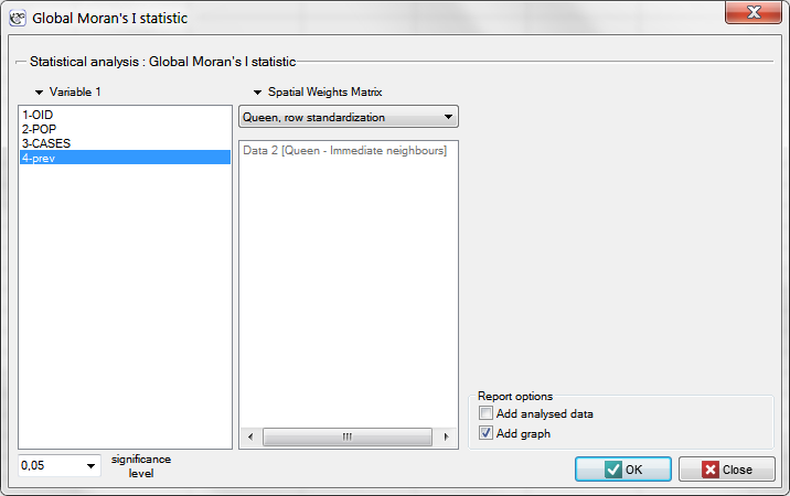
Example 3. (catalog: leukemia, file: leukemia.pqs) The analysis will concern the data gathered and analyzed by L.A. Waller and others in 1992[12] and 1994[13], described on 281 objects in 2004[14].
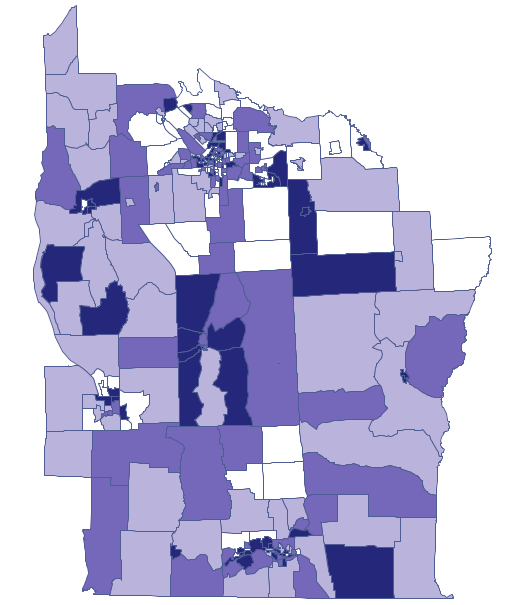
Epidemiologically interesting are the regions in which the prevalence of leukemia is higher, as their grouping could indicate the existence within their boundaries of environmental teratogens causing an increased frequency of occurrence of leukemia.
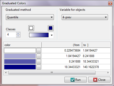
We start from presenting the geographic distribution of the frequency coefficient (prev) on the map. For that purpose we draw a map in the Map Manager and edit the layer  , choosing Graduated colors:
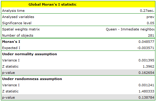
Moran's correlation coefficient obtained in the analysis is small and has the value \(I=0.048577\):
Global Geary's C statistic
Similarly to Moran's analysis, global Geary's statistic studies the degree of the intensity of a given feature in spatial objects.
Note
It is not recommended to conduct Geary's analysis for objects without a neighborhood (objects described in a weight matrix only with the value 0). Such objects can be excluded from the analysis by deactivating them (Chapter ?), or the analysis can be made with the use of a different manner of defining neighborhood (a different weight matrix).
- Geary's autocorrelation coefficient
– introduced by Geary in 1954 [7].
It is one of the possible alternatives for the global Moran's statistic. Similarly to Moran's analysis, Geary's statistic studies the degree of intensity of a given \(x_i\) feature in spatial objects described with the use of a weight matrix with \(w_{ij}\) elements. This time, instead of computing the sum of quotients: \(\sum\sum w_{ij}(x_i-\overline{x})(x_j-\overline{x})\) we compute the sum of the difference squares:\[ \sum\sum w_{ij}(x_i-x_j)^2 \]As a result, Geary's autocorrelation coefficient is expressed with the formula:
\[ c=\frac{\sum_{i=1}^n\sum_{j=1}^nw_{ij}(x_i-x_j)^2}{2 S_0 sd^2} \]where:
\(n\) – the number of spatial objects (the number of points or polygons),
\(x_i\), \(x_j\) – are the values of the variable for the compared objects,
\(w_{ij}\) – elements of the spatial weights matrix (weights matrix row standardized),
\(S_0=\sum_{i=1}^n\sum_{j=1}^nw_{ij}\),
\(sd^2=\frac{\sum_{i=1}^n\left(x_i-\overline{x}\right)^2}{n-1}\) – variance,
\(\overline{x}\) – it is the mean value of the variable for all objects.The interpretation of Geary's coefficient:
- \(c<1\) and \(c \approx 0\) means the occurrence of clusters with similar values – a positive autocorrelation;
- \(c>1\) means the occurrence of the so-called hot spots, i.e. distinctly different values in neighboring areas – a negative autocorrelation;
- \(c \approx 1\) means a random spatial distribution of the studied variable – a lack of autocorrelation.
Note
When the values of a studied feature are characterized by a great variability of variance then it is desirable to stabilize that variability. The basic information about smoothing variables have been described in the Chapter SPATIAL SMOOTHING SPATIAL SMOOTHING- Significance of Geary's autocorrelation coefficient
A test for checking the significance of Geary's autocorrelation coefficient serves the purpose of verifying the hypothesis about a lack of spatial autocorrelation
Hypotheses:\(\begin{array}{cl} \mathcal{H}_0: & C = 1, \\ \mathcal{H}_1: & C \ne 1. \end{array}\)
The test statistic has the form presented below:
\[ Z=\frac{C-E(C)}{\sqrt{var(C)}}, \]where:
\(\displaystyle E(C)=1\) – the expected value,
\(\displaystyle var(C)\) – variance.
Depending on the assumption concerning the distribution of the population from which the sample has been taken, the manner of selecting variance is chosen (Cliff and Ord (1981)[5], and Goodchild (1986)[8]). If it is a normal distribution, then:\[ var(C)=\frac{(2S_1+S_2)(n-1)-4S_0^2}{2(n+1)S_0^2}, \]where:
\(S_1\) and \(S_2\) are defined as for Moran's analysis.If it is a random distribution, then:
\(var(CS)=\frac{(n-1)S_1\left(n^2-3n+3-(n-1)b_2\right)-(n-1)S_2\left(n^2+3n-6-(n^2-n+2)b_2\right)\frac{1}{4}+S_0^2\left(n^2-3-(n-1)^2b_2\right)}{n(n-2)^{(2)}S_0^2},\)where:
\(b_2=\frac{\frac{1}{n}\sum_{i=1}^n\left(x_i-\overline{x}\right)^4}{\left(\frac{1}{n}\sum_{i=1}^n\left(x_i-\overline{x}\right)^2\right)^2}\),
\(n^{(b)}=n(n-1)(n-2)...(n-b+1)\).Statistics \(Z\) has, asymptotically (for large sample sizes), normal distribution.
On the basis of test statistics, \(p\) value is estimated and then compared with the significance level \(\alpha\) :\[ \begin{array}{ccl} \text{ if } p \le \alpha & \Longrightarrow & \text{ we reject } \mathcal{H}_0 \text{ and accept } \mathcal{H}_1, \\ \text{ if } p > \alpha & \Longrightarrow & \text{ there is no reason to reject } \mathcal{H}_0. \\ \end{array}\]
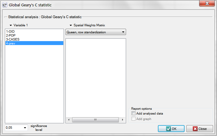
The window with settings for Geary's analysis is accessed via the men Spacial analysis \(\to\) Spacial statistics \(\to\) Global Geary's C statistic.
Example 3 cont. (catalog: leukemia, file: leukemia)
We will analyze the data concerning leukemia.
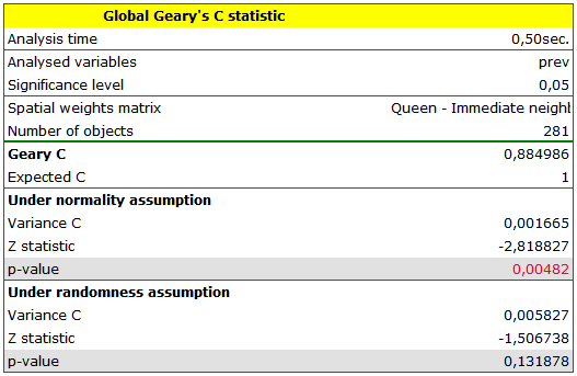
Global Moran's analysis has pointed to a lack of spatial autocorrelation. This time, in order to check if in the studied area of the northern part of the state of New York it is possible to localize clusters of leukemia we will compute the global Geary's C statistic.
We start from the presentation of the geographic distribution of the prevalence coefficient (prev) on the map, according to the values of the prev variable, dividing it into quartiles:
LOCAL ESTIMATE OF SPATIAL CLUSTERING
In the local analysis we try to define clusters according to their placement, size, and intensity. A cluster is understood as a limited gathering of objects of certain intensity, placed in space and/or time, an accidental appearance of which is highly improbable. If we identify such a gathering which is not accidental but is a statistically significant cluster we can infer the reasons for its occurrence.
Local Moran's I statistic
Local Moran's I statistic is the most popular analysis from those defined as LISA (Local Indicators of Spatial Association) (Luc Anselin 1995 [1]). In contrast to Global Moran's I statistic it defines the local spacial autocorrelation, i.e. defines the similarity of a spatial unit to its neighbors and studies the statistical significance of that dependence.
- Local Moran's I coefficient
The local form of Moran's \(I\) coefficient for the \(i\) observation is defined with the formula:\[ I_i=\frac{\left(x_i-\overline{x}\right)\sum_{j=1}^nw_{ij}\left(x_j-\overline{x}\right)}{\sigma^2} \]where:
\(n\) – the number of spatial objects (the number of points or polygons),
\(x_i\), \(x_j\) – are the values of the variable for the compared objects,
\(\overline{x}\) – it is the mean value of the variable for all objects,
\(w_{ij}\) – elements of a spacial weight matrix (it is recommended that the matrix is row standardized),
\(\sigma^2=\frac{\sum_{i=1}^n\left(x_i-\overline{x}\right)^2}{n-1}\) – varianceThe interpretation of the local Moran's coefficient is analogous to its global counterpart, however, it largely depends on the selected weight matrix. Most often non-zero matrices are ascribed only to neighboring objects. As a result the local coefficient only describes the similarity of objects in the zone of neighborhood. Row standardization makes it easier to compare the values of coefficients obtained for various objects as the expected value for each coefficient is then the same.
High values of a coefficient point to the occurrence of clusters with similar values while low values of a coefficient point to the occurrence of the so-called hot spots, and values near the expected value \(E(I_i)\) point to the random distribution in space of the studied variable.
The expected value is defined with the formula:\[ E(I_i)=\frac{-\sum_{j=1}^nw_{ij}}{n-1} \]- The significance of Moran's autocorrelation coefficient
By testing the statistical significance of the relationship among the neighboring objects the following hypotheses are studied:\(\begin{array}{cl} \mathcal{H}_0: & I_i = E(I_i), \\ \mathcal{H}_1: & I_i \ne E(I_i). \end{array}\)
The test statistic has the form presented below:
\[ Z_i=\frac{I_i-E(I_i)}{\sqrt{var(I_i)}}, \]where:
\(\displaystyle var(I_i)=\frac{w_{i(2)}(n-b_2)}{n-1}+\frac{2w_{i(kh)}(2b_2-n)}{(n-1)(n-2)}-\frac{\left(\sum_{j=1}^nw_{ij}\right)^2}{(n-1)^2}\) – variance in a random distribution,\(b_2=\frac{(n-1)\sum_{i=1}^n\left(x_i-\overline{x}\right)^4}{\left(\sum_{i=1}^n\left(x_i-\overline{x}\right)^2\right)^2}\),
\(w_{i(2)}\) – the sum of weights square for the \(i\) row,
\(2w_{i(kh)}\) – the sum of possible weights ratios for the \(i\) row, after the exclusion of ratios with the same indexes.The \(Z_i\) statistics has, asymptotically (for large sample sizes), normal distribution.
On the basis of test statistics, \(p\) value is estimated and then compared with the significance level \(\alpha\) :\[ \begin{array}{ccl} \text{ if } p \le \alpha & \Longrightarrow & \text{ we reject } \mathcal{H}_0 \text{ and accept } \mathcal{H}_1, \\ \text{ if } p > \alpha & \Longrightarrow & \text{ there is no reason to reject } \mathcal{H}_0. \\ \end{array}\]Due to the problem of a lack of independence of coefficients computed for neighboring objects it is suggested to use a corrected significance level \(\alpha\). The suggested corrections are: Bonferroni correction: \(\alpha_1=\alpha/k\) or Šidák correction: \(\alpha_1=1-(1-\alpha)^{1/k}\), where \(k\) is the arithmetic mean number of the neighbors.
- Map layers
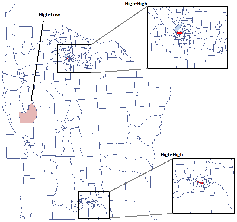
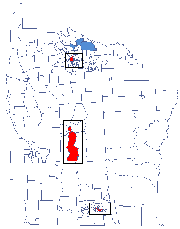
The combination of information from Moran's scatter plot (the division of objects into: High-High, Low-Low, Low-High, High-Low) and from the significance of the local Moran's statistics presents on a map the so-called spatial regimes:- Statistically significant High-High objects (objects with high values surrounded by objects with high values) are marked in red on the map;
- Statistically significant Low-Low objects (objects with low values surrounded by objects with low values) are marked in blue on the map;
- Statistically significant Low-High objects (objects with low values surrounded by objects with high values) are marked in light blue on the map;
- Statistically significant High-Low objects (objects with high values surrounded by objects with low values) are marked in light red on the map.
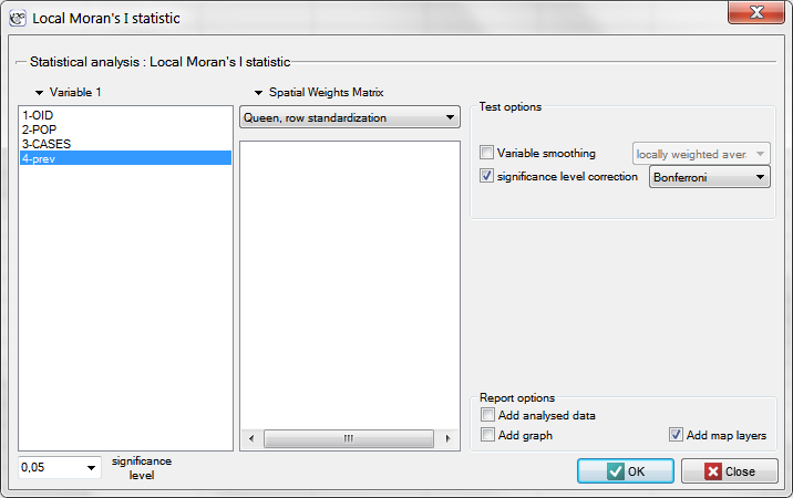
The window with the settings of the local Moran's analysis option is accessed via the menu Spatial analysis \(\to\) Spatial statistics \(\to\) Local Moran's I statistic.
Example 3 cont. (catalog: leukemia, file: leukemia)
We will analyze data about leukemia.
The global analysis has not yielded an unambiguous answer as to the occurrence of spatial autocorrelation. We will, then, check if we can find regions in which the prevalence of leukemia is significantly higher.
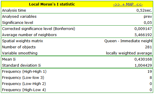
In order to localize clusters of leukemia and regions which contrast with the environment with respect to the prevalence of that disease we will compute the local Moran's coefficient. For the analysis we will use the prev variable and the neighborhood matrix – Queen, row standardized (according to the contiguity) which is suggested by the program. In order to use a different matrix one has to generate it first, see chapter: Spatial weight matrix. We also select one of the corrections of the significance level.
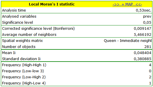 ) – those are spatial regimes described in the report with the use of the color column.
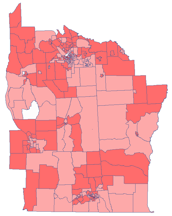
The obtained results can be further illustrated when the map is colored with the values of the local Moran's \(I_i\) coefficient or the values of a test statistic, or \(p\) values. One just has to copy the appropriate columns from the report into a datasheet. In this example we will use the values of the \(Z(I_i)\) test statistic for coloring. Having pasted it into an empty column of a datasheet, in the map manager we color the base map according to the values of that column, selecting the standard deviation with the coefficient 3 as a way of gradiating colors. Positive and high values of the \(Z_i\) statistics point to the occurrence of clusters of similar values while negative and low values of that statistic point to the occurrence of the so-called hot spots. Values close to 0 point to a random distribution of the studied value in space.
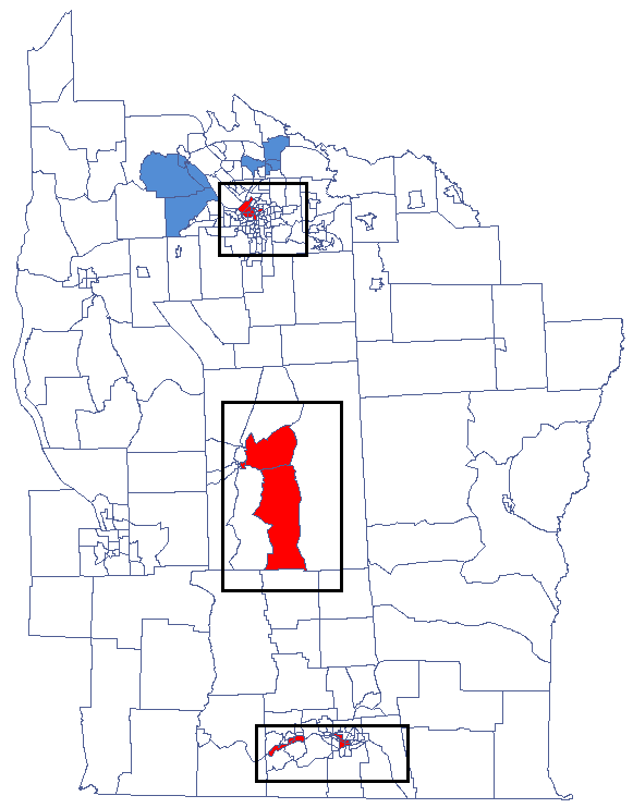
Local Getis-Ord’s G statistic
Getis and Ord's \(G_i\) statistic (Getis and Ord 1992, Ord and Getis 1995) allows the detection of a local concentration of high and low values in neighboring objects and studies the statistical significance of that dependence. Getis and Ord have also defined a \(G^*_i\) statistics, very similar to the \(G_i\) statistics. The only difference between them is that in the case of the former the object for which the study is made also takes part in the analysis. In a weight matrix, then, the so-called potential is defined for that object, i.e. the neighborhood with itself (values on the axis are greater than 0).
- Getis-Ord’s G coefficient
The local form of Getis and Ord's \(G\) coefficient for the \(i\) observation is defined with the formula:\[ G_i=\frac{\sum_{j=1}^nw_{ij}x_j}{\sum_{j=1}^nx_j}, \quad \textrm{where: $i\neq j$.} \]The \(G^*_i\) coefficient is defined with the same formula but the computations are also made for the studied object, that is the object for which the \(i\) and the \(j\) indexes are equal.
As the coefficient is based on a quotient of two sums of the values of the (\(x_j\)) objects, in order to interpret the coefficient correctly it is important that the analyzed phenomenon is described with the use of positive numbers. The interpretation of Getis and Ord's local coefficient, similarly to local Moran's coefficient, depends, to a great degree, on the selected weight matrix (row standardization of the matrix is recommended). High values of the \(G_i\) or \(G^*_i\) coefficients point to a concentration of objects with high values of the analyzed phenomenon, whereas low values point to a clustering of objects with low values. When the values are close to the expected value then the spatial distribution of the studied value is random.
The expected value is defined with the formula:\[ E(G_i)=\frac{\sum_{j=1}^nw_{ij}}{n-1}, \quad \textrm{where: $i\neq j$}; \]\[ E(G_i^*)=\frac{\sum_{j=1}^nw_{ij}}{n}. \]- The significance of Getis and Ord's coefficient
By testing the statistical significance of the relationship among the neighboring objects the following hypotheses are studied:\(\begin{array}{clccl} \mathcal{H}_0: & G_i = E(G_i) & \quad & \mathcal{H}_0: & G_i^* = E(G_i^*)\\ \mathcal{H}_1: & G_i \ne E(G_i), & \quad & \mathcal{H}_1: & G_i^* \ne E(G_i^*). \end{array}\)
The test statistic has the form presented below:
\[ Z_i(G)=\frac{\sum_{j=1}^nw_{ij}x_j-\overline{x}(i)\sum_{j=1}^nw_{ij}}{s(i)\sqrt{\frac{(n-1)\sum_{j=1}^nw_{ij}^2-\left(\sum_{j=1}^nw_{ij}\right)^2}{n-2}}}, \quad \textrm{where: $i\neq j$}; \]\[ Z_i(G*)=\frac{\sum_{j=1}^nw_{ij}x_j-\overline{x}^*\sum_{j=1}^nw_{ij}}{s^*\sqrt{\frac{n\sum_{j=1}^nw_{ij}^2-\left(\sum_{j=1}^nw_{ij}\right)^2}{n-1}}}. \]where:
\(\overline{x}(i)\) i \(\overline{x}^*\) – the mean of the variable \(X\),
\(s(i)^2\) i \(s^{*2}\) – the variance of the \(X\) variable.The \(Z_i\) statistics has, asymptotically (for large sample sizes), normal distribution.
On the basis of test statistics, \(p\) value is estimated and then compared with the significance level \(\alpha\) :\[ \begin{array}{ccl} \text{ if } p \le \alpha & \Longrightarrow & \text{ we reject } \mathcal{H}_0 \text{ and accept } \mathcal{H}_1, \\ \text{ if } p > \alpha & \Longrightarrow & \text{ there is no reason to reject } \mathcal{H}_0. \\ \end{array}\]Due to the problem of a lack of independence of coefficients computed for neighboring objects it is suggested to use a corrected significance level \(\alpha\). The suggested corrections are: Bonferroni correction: \(\alpha_1=\alpha/k\) or Šidák correction: \(\alpha_1=1-(1-\alpha)^{1/k}\), where \(k\) is the arithmetic mean number of the neighbors.
- Map layers
The combination of the information from the value of the \(Z_i\) statistic and its significance presents the so-called spacial regimes on the map:- Statistically significant objects with high values of the \(Z_i\) statistic are marked as High-High (objects with high values surrounded by objects with high values) and marked in red on the map;
- Statistically significant objects with low values of the \(Z_i\) statistic are marked as Low-Low (objects with low values surrounded by objects with low values) and marked in blue on the map;
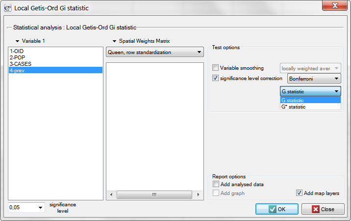
The window with settings for Local Getis and Ord's analysis is accessed via the menu Spatial analysis \(\to\) Spatial statistics \(\to\) Getis-Ord \(G_i\) statistic.
Example 3 cont. (catalog: leukemia, file: leukemia)
We will analyze the data concerning leukemia.
The global analysis has not yielded an unambiguous answer as to the occurrence of spatial autocorrelation. We will, then, check if we can find regions in which the prevalence of leukemia is significantly higher.
In order to localize leukemia clusters we will compute the \(G_i\) and \(G_i^*\) coefficients. The analysis will be conducted with the prev variable and the neighborhood matrix – Queen, row standardized (according to contiguity) which is suggested by the program. In order to use a different matrix one has to generate it first, see chapter: Spatial weight matrix. We also select one of the corrections of the significance level.
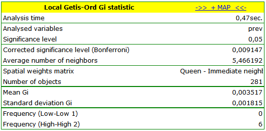
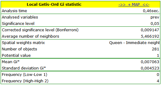 ) – those spatial regimes are defined in the report with the use of the color column.
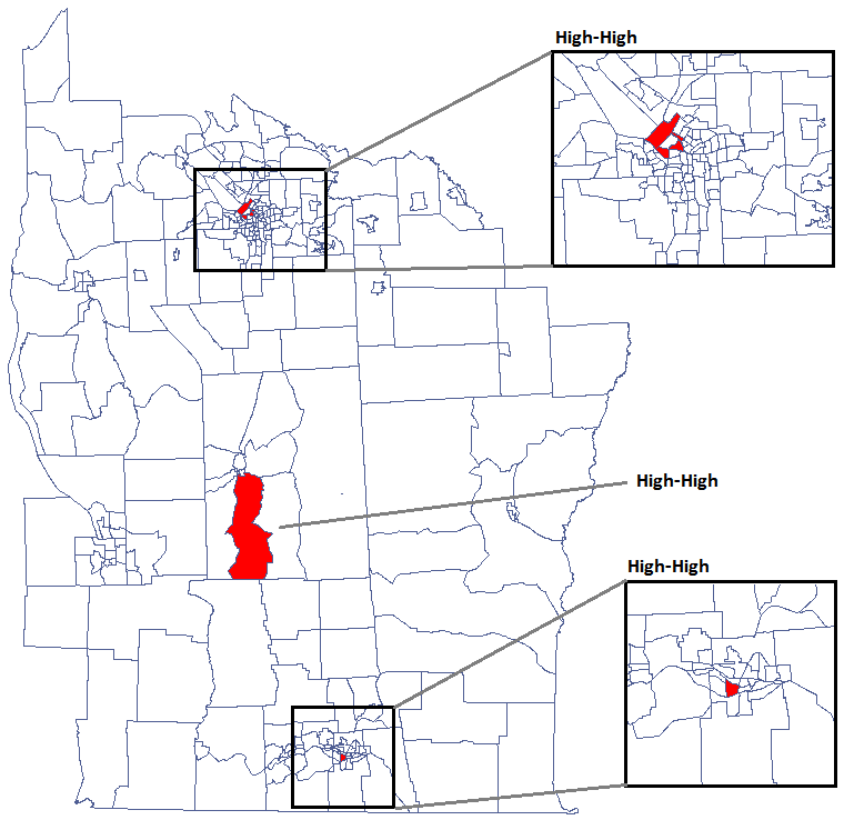
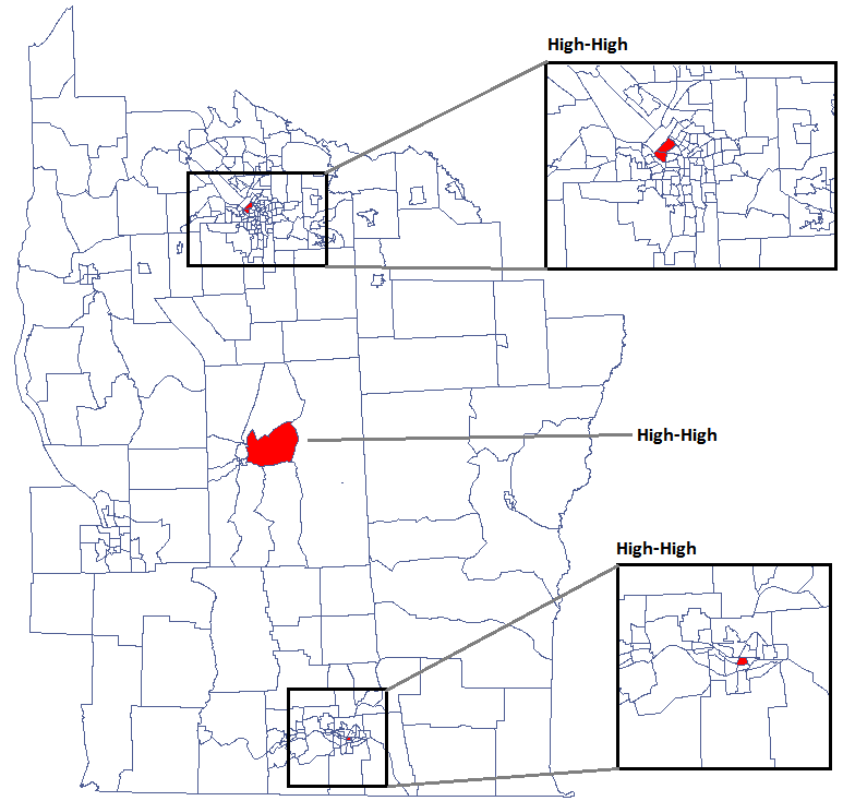
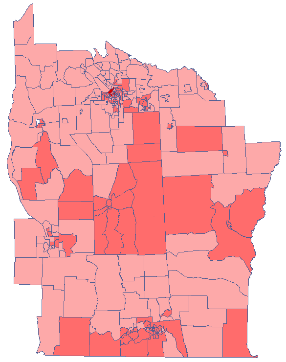
The obtained results can be additionally illustrated by coloring the map so as to present the values of the local Getis and Ord's coefficient or the values of the test statistic, or the \(p\) values. One just has to copy the appropriate columns from the report and paste them into a datasheet. In this example we will use the values of the \(Z(G_i)\) test statistic for coloring. Having pasted it into an empty column of a datasheet, in the map manager we color the base map according to the values of that column, selecting the standard deviation with the coefficient 3 as a way of gradiating colors. Positive and high values of the \(Z_i\) statistic point to a concentration of objects with high values, whereas negative and low values point to a concentration of objects with low values, and the values near zero point to a random spatial distribution of the studied variable (a map can be added with means and confidence intervals).
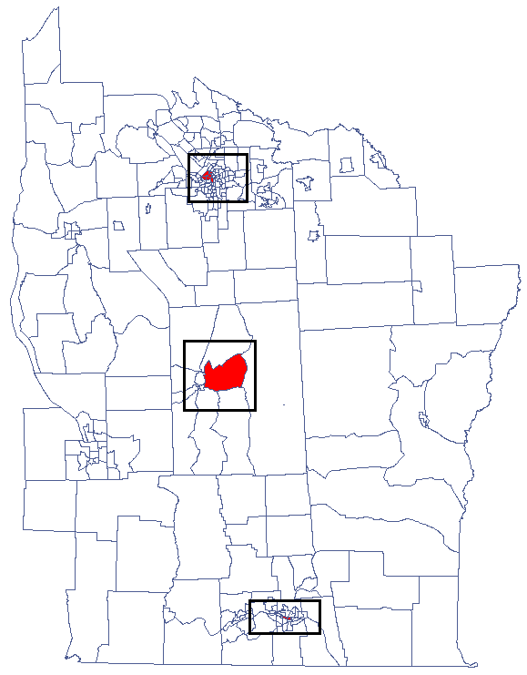
CutL
CutL method was developed to detect clusters that have significantly higher prevalence than that specified by the investigator[15]. As a result, the program locates clusters, examines their statistical significance, and plots them on a map.
Note
Analysis is based on the commonly used Binomial test for equal proportions.
Analyses are conducted on aggregated data (polygons map). In each of the two columns of the data sheet, enter the population size and number of cases for EACH object – these are the data required for proper analysis.
| ID | Pop | Cases |
| 1 | 548028 | 505 |
| 2 | 4896 | 2 |
| 3 | 3981 | 5 |
| 4 | 5658 | 7 |
| 5 | 9591 | 4 |
| 6 | 3011 | 2 |
| 7 | 4938 | 7 |
| 8 | 8664 | 11 |
| … | … | … |
| … | … | … |
The settings window of CutL statistic can be opened in Spatial analysis\(\to\)Spatial statistics\(\to\)CutL
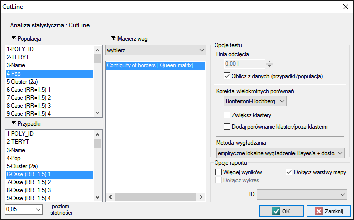
The analysis is based on data from the population size and number of cases, as well as the neighborhood matrix on the map.
Using the neighborhood matrix:
The Queen neighborhood matrix is the default chosen during the analysis. Other matrices may be used in this analysis, but this requires prior preparation and selection in the analysis window.
The cut-off line is the value above which statistically significant clusters can be detected and may be set in the analysis window. If the investigator does not specify this value, then it is set to the average prevalence calculated for the area under study.
Options
Corrections for multiple comparisons
The following corrections for multiple comparisons may be used:- Bonferroni-Hochberg
- Sidak-Hochberg
- Benjamini-Hochberg
Compare cluster/outside In addition, each cluster may be compared with the area outside of the cluster. The Binomial test for one proportion compares the prevalence within the cluster to the specified prevalence value, which is the prevalence outside of the cluster. Hypothesis testing is one-sided resulting from the higher prevalence inside the cluster than outside.
Results of Analysis
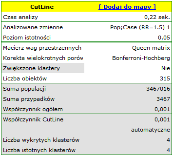
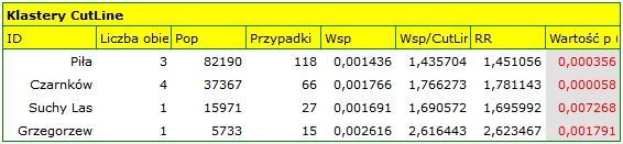
The results of the analysis are presented in the form of a report and map with superimposed layers.
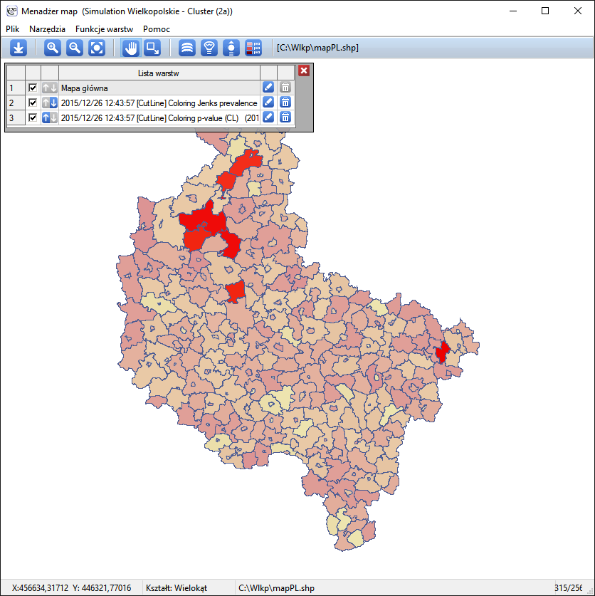
Spatial-Temporal CutL
sing the CutL method, it is also possible to determine temporal-spatial clusters (Więckowska B. 2019 [16]), i.e., clusters that do not persist for the entire time range under study, but only for a shorter period.
Individual time layers are added to the datasheet by selectingr Edit Timeline from the project tree, after indicating the appropriate map.
The spatio-temporal analysis window is obtained by selecting the menu Spatial analysis\(\to\)Spatial statistics\(\to\)CutL space-time.
- Anselin L., (1995), Local Indicators of Spatial Association – LISA; Geographical Analysis, 27(2): 93–115
- Anselin L., Lozano N., Koschinsky J. (2006) Rate Transformations and Smoothing. GeoDa Center Research Report https://geodacenter.asu.edu
- Buliung R.N., Remmel T.K. (2008), Open source, spatial analysis, and activity-travel behaviour research: capabilities of the aspace package. Journal of Geographical Systems 10, 191-216
- Clark P.J., Evans F.C. (1954), Distance to nearest neighbour as a measure of spatial relationships in populations. Ecology 35, 445-453.
- Cliff A.D., Ord J.K., (1981), Spatial Processes: Models and Applications. Pion: London.
- Fisher R.A. (1936), The use of multiple measurements in taxonomic problems. Annals of Eugenics, 7:179-188.
- Geary R.C., (1954), The Contiguity Ratio and Statistical Mapping. The Incorporated Statistician, 5, 115-45
- Goodchild M.F., (1986), Spatial Autocorrelation, CATMOG 47, Geobooks: Norwich UK
- Moran P.A.P., (1947), The Interpretation of Statistical Maps. Journal of the Royal Statistical Society, B10, 243-51
- O'Rourke J. (1998), Computational Geometry in C (2nd ed). Massachusetts: Smith College
- De Smith M.J., Goodchild M.F., Longley P.A. (2007) Geospatial Analysis, A Comprehensive Guide to Principles, Techniques and Software Tools (2nd ed). Matador
- Waller L.A., Turnbull B.W., Clark L.C., Nasca P., (1992), Chronic disease surveillance and testing of clustering of disease and exposure : Application to leukemia incidence and TCE-contaminated dumpsites in upstate New York. Environmetrics, 3, 281-300
- Waller L.A., Turnbull B.W., Clark, L.C., Nasca P., (1994), Spatial pattern analyses to detect rare disease clusters, in Case Studies in Biometry, N. Lange, et al., Editors. , John Wiley and Sons: New York, 3-23
- Waller L.A., Gotway C.A., (2004) Applied Spatial Statistics for Public Health Data. New York: John Wiley and Sons
- Więckowska B., Marcinkowska J. (2017), CutL: an alternative to Kulldorff’s scan statistics for cluster detection with a specified cut-off level. Geospatial Health, 12(2): 556
- Więckowska B., Górna I., Trojanowski M., Pruciak A., Stawińska-Witoszyńska B. (2019), Searching for space-time clusters: The CutL method compared to Kulldorff's scan statistic 14(2)
- Yamamoto J.K. (1997), A Pascal program for determining the convex hull for planar sets. Computers and Geosciences 23, n. 7, 725-738