The Skillings-Mack ANOVA (missing data)

When to use this test:

The analysis of variance of repeated measurements for Skillings-Mack ranks (Skillings and Mack, 1981[157]) is used in the same situation as the Friedman ANOVA, but when the data contain gaps that do not follow any particular pattern (each object only needs at least two observations). When there are no gaps and no tied ranks, the test is identical to the Friedman ANOVA; when gaps occur in a balanced arrangement, it gives the same results as the Durbin ANOVA.

Assumptions

measurement on an ordinal scale or an interval scale,
a dependent model,
each object has at least two observations.

How to set up the analysis

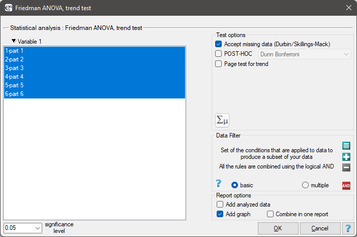
Statistics \(\to\) Nonparametric tests (ordered categories) \(\to\) Friedman ANOVA (missing data allowed).

Step 1. Select the variables corresponding to successive measurements.

Step 2. Select the Accept missing data option.

Step 3. Run the analysis.

Note! For records with missing data to be taken into account, the Accept missing data option must be selected. Empty cells and cells with non-numeric values are treated as missing data. Only records containing more than one numeric value are included in the analysis. There is no POST-HOC analysis available for this test.

Performing and interpreting the analysis

Example 1. (polling.pqs file)
A university teacher, wanting to improve the way he conducted his classes, decided to verify his teaching skills. In several randomly selected student groups, during the last class, he asked students to fill in a short, anonymous questionnaire consisting of 6 questions about how six specified parts of the course material were illustrated (five-point scale, where 1 – a completely incomprehensible way of presenting the material, 5 – a very clear and interesting way of illustrating the material). The data obtained turned out to be incomplete: in the 30-person group completing the survey, only 15 people provided a complete set of answers. An analysis that does not take the gaps into account (Friedman ANOVA) would have limited power due to such a drastic reduction in group size. The gaps were also not planned and do not form a balanced block, so the Durbin ANOVA cannot be used either. We will check whether the ratings of the individual parts of the material differ from one another.

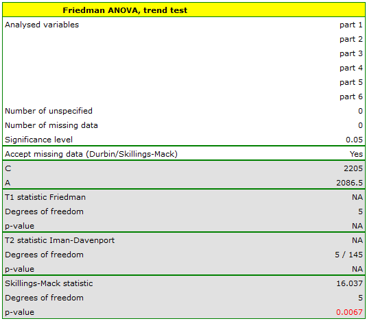
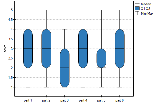
\(p=0.006739\) (statistically significant, \(\alpha=0.05\))

The ratings of the individual parts of the material differ statistically significantly.

The obtained \(p\) value should be treated with caution due to possible tied ranks – in this case, however, it is well below the assumed significance level. The differences in responses can be observed in the graph; there is no POST-HOC analysis available for this test.

FOR THOSE INTERESTED

Hypotheses: they relate to the equality of the sum of ranks for successive measurements (\(R_j\)) or are simplified to medians (\(\theta_j\)):

\[\begin{array}{cl} \mathcal{H}_0: & \theta_1=\theta_2=...=\theta_k,\\ \mathcal{H}_1: & \text{not all }\theta_j\text{ are equal }(j=1,2,...,k), \end{array}\]

Formulas: the test statistic is defined by:

\[ \chi^2=A\Sigma_0^{-1}A^T, \]

where:
\(A=(A_1,A_2,...,A_{k-1})\),
\(A_j=\sum_{i=1}^n\sqrt{\frac{12}{s_i+1}}\left(R_{ij}-\frac{s_i+1}{2}\right)\),
\(s_i\) – number of observations for object \(i\),
\(R_{ij}\) – ranks assigned to successive measurements (\(j=1,2,...k\)), separately for each object studied (\(i=1,2,...n\)), with ranks for missing data equal to the mean rank for that object,
\(\Sigma_0\) – matrix determining the covariances of \(A\) under \(\mathcal{H}_0\)[157].

When each pair of measurements occurs simultaneously for at least one observation, this statistic asymptotically (for large sample sizes) has the \(\chi^2\) distribution with \(k-1\) degrees of freedom.

The \(p\) value, determined on the basis of the test statistic, is compared with the significance level \(\alpha\): if \(p \le \alpha\), we reject \(\mathcal{H}_0\) in favor of \(\mathcal{H}_1\); if \(p > \alpha\), there is no reason to reject \(\mathcal{H}_0\).