 PQStat
Multiple linear regression
When to use:
The constructed multiple regression model allows the study of the influence of many independent variables (\(X_1\), \(X_2\), \(\ldots\), \(X_k\)) on one dependent variable (\(Y\)). The most frequently used variety of multiple regression is Multiple Linear Regression. It is an extension of linear regression models based on the Pearson product-moment correlation coefficient. It assumes the existence of a linear relationship between the variables studied. The linear multiple regression model takes the form:
where:
\(Y\) – the dependent variable, explained by the model,
\(X_1,X_2,\ldots X_k\) – independent, explanatory variables,
\(\beta_0,\beta_1,\beta_2,\ldots \beta_k\) – parameters,
\(\epsilon\) – the random component (model residual).
Assumptions
- measurement of the dependent variable \(Y\) on an interval scale,
- a linear relationship between the dependent and independent variables,
- a sufficiently large number of observations.
Definitions of measures
Dummy variables and interactions in the model – a discussion of the preparation of dummy variables and interactions is presented in section Preparation of variables for analysis in multivariate models Preparation of variables for analysis in multivariate models.
Regression coefficients – if the model was built using a sample of size \(n\), the above equation can be represented in matrix form:
where: \( Y=\left( \begin{array}{ccc} y_1\\ y_2\\ \vdots\\ y_n \end{array} \right), \) \( X=\left( \begin{array}{ccccc} 1 & x_{11} & x_{21} & \ldots & x_{k1}\\ 1 & x_{12} & x_{22} & \ldots & x_{k2}\\ \vdots & \vdots & \vdots & \ddots & \vdots\\ 1 & x_{1n} & x_{2n} & \ldots & x_{kn} \end{array} \right), \) \( \beta=\left( \begin{array}{ccc} \beta_0\\ \beta_1\\ \beta_2\\ \vdots\\ \beta_k \end{array} \right), \) \( \epsilon=\left( \begin{array}{ccc} \epsilon_1\\ \epsilon_2\\ \vdots\\ \epsilon_n \end{array} \right). \)
The solution of the equation is then the vector of parameter estimates \(\beta_0,\beta_1,\ldots,\beta_k\), called the regression coefficients:
\( b=\left( \begin{array}{ccc} b_0\\ b_1\\ b_2\\ \vdots\\ b_k \end{array} \right). \)
These coefficients are estimated using the classical least squares method. On the basis of these values, we can draw conclusions about the magnitude of the effect of the independent variable (for which the coefficient was estimated) on the dependent variable – they tell us by how many units the dependent variable will change when the independent variable changes by 1 unit. Each coefficient carries a certain estimation error, calculated from the formula \(SE_b=\sqrt{\frac{1}{n-(k+1)}e^Te(X^TX)^{-1}}\), where \(e=Y-\widehat{Y}\) is the vector of model residuals (the difference between the actual values of the dependent variable \(Y\) and the values \(\widehat{Y}\) predicted from the model).
How to set up the analysis
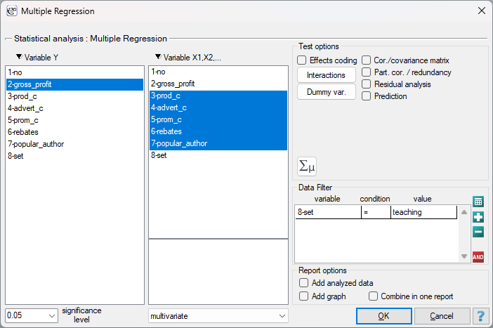
Advanced statistics \(\to\) Multivariate models \(\to\) Multiple regression.
Model verification
Statistical significance of individual variables in the model – on the basis of the coefficient and its estimation error, we can infer whether the independent variable for which this coefficient was estimated has a significant effect on the dependent variable. For this purpose, we use the \(t\)-test.
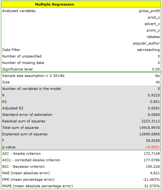
Quality of the constructed model – the quality of a multiple linear regression model can be assessed using several measures:
- Standard error of estimation – a measure of model fit, based on the model residuals \(e_i=y_i-\widehat{y}_i\), i.e. the discrepancy between the actual values of the dependent variable \(y_i\) in the sample and the values of the dependent variable \(\widehat{y}_i\) calculated from the constructed model. For the model to be well fitted, the standard error of estimation should be as small as possible.
- Multiple correlation coefficient \(R=\sqrt{R^2} \in \langle0; 1\rangle\) – indicates the strength of the effect of the set of variables \(X_1,X_2,\ldots X_k\) on the dependent variable \(Y\).
- Multiple coefficient of determination \(R^2\) – a measure of model fit. The value of this coefficient falls within the range \(\langle0; 1\rangle\), where 1 means a perfect fit and 0 means a complete lack of fit. It expresses the percentage of variability in the dependent variable explained by the model. Since the value of \(R^2\) depends on the model fit but is also sensitive to the number of variables in the model and the sample size, an adjusted value \(R^2_{adj}\) is also calculated.
- Information criteria (\(AIC\), \(AICc\), \(BIC\)) – based on the entropy of the information carried by the model (the model's uncertainty), i.e. they estimate the information lost when a given model is used to describe the phenomenon studied. We should choose the model with the minimum value of the given information criterion. An information criterion is not, however, an absolute measure – if all the models compared describe reality poorly, looking for a warning sign in the information criterion makes no sense.
- Error analysis for ex post forecasts (\(MAE\), \(MPE\), \(MAPE\)) – describe the accuracy of the forecast, indicating on average how much the actual realisations of the dependent variable will deviate from the forecasts.
- Statistical significance of all variables in the model – the basic tool for estimating the significance of all variables in the model is the analysis of variance test (F-test).
More information about the variables in the model:
- Standardized \(b_1,b_2,\ldots,b_k\) – unlike raw parameters (which, depending on the variable described, are expressed in different units of measurement and cannot be directly compared), standardized parameter estimates allow the contribution of individual variables to explaining the variability of the dependent variable \(Y\) to be compared.
- Correlation matrix – contains information about the strength of the relationship between individual variables, i.e. the Pearson correlation coefficient \(r_p \in \langle-1; 1\rangle\), calculated for each pair of variables, without taking into account the influence of the other variables in the model.
- Covariance matrix – like the correlation matrix, contains information about the linear relationship between individual variables, except that this value is not standardized.
- Partial correlation coefficient – falls within the range \(\langle-1; 1\rangle\) and is a measure of the correlation between a specific independent variable \(X_i\) (taking into account its correlation with the other variables in the model) and the dependent variable \(Y\) (taking into account its correlation with the other variables in the model). The square of this coefficient is the partial coefficient of determination – falls within the range \(\langle0; 1\rangle\) and represents the ratio of the exclusive variability of a given independent variable \(X_i\) to the variability of the dependent variable \(Y\) that has not been explained by the other variables in the model. The closer these coefficients are to 0, the more useless the information carried by the variable studied, i.e. the more redundant it is.
- Semi-partial correlation coefficient – falls within the range \(\langle-1; 1\rangle\) and is a measure of the correlation between a specific independent variable \(X_i\) (taking into account its correlation with the other variables in the model) and the dependent variable \(Y\) (NOT taking into account its correlation with the other variables in the model). The square of this coefficient is the semi-partial coefficient of determination – falls within the range \(\langle0; 1\rangle\) and represents the ratio of the exclusive variability of a given independent variable \(X_i\) to the total variability of the dependent variable \(Y\).
- R-squared (\(R^2 \in \langle0; 1\rangle\)) – expresses the percentage of variability in a given independent variable \(X_i\) explained by the other independent variables. The closer to 1, the more strongly the variable studied is linearly related to the other independent variables, which may mean it is a redundant variable.
- Variance inflation factor (\(VIF \in \langle1; \infty)\)) – indicates how much the variance of the estimated regression coefficient is increased due to collinearity. The closer to 1, the lower the collinearity. Strong collinearity is assumed to occur when \(VIF>5\)[153].
- Tolerance \(=1-R^2 \in\langle0; 1\rangle\) – expresses the percentage of variability in a given independent variable \(X_i\) NOT explained by the other independent variables. The closer the tolerance value is to 0, the more strongly the variable studied is linearly related to the other independent variables, which may mean it is a redundant variable.
- Comparison of the full model with the model after removing a given variable – performed using the F-test (when more than one variable is removed from the model) or the \(t\)-test (when only one variable is removed – this is the same test used to examine the significance of individual variables in the model; the results of both tests are then identical). If the difference between the compared models is statistically significant, the full model is significantly better than the reduced model, which means the variable studied is not redundant.
- Scatter plots – allow a subjective assessment of the linearity of the relationship between variables and the identification of outliers, and can also be used in the analysis of model residuals.
Analysis of model residuals
To obtain a correct regression model, we should check the basic assumptions concerning the model residuals:
- Outliers – examining the model residuals quickly gives us information about outlying values. Such observations can greatly disturb the regression equation, since they have a large influence on the values of its coefficients. If a given residual \(e_i\) is more than 3 standard deviations from the mean value, it may be suspected that removing this observation will improve the model. Cook's distance describes the magnitude of changes in the regression coefficients resulting from omitting a given case (in the program, Cook's distances are marked in bold for cases exceeding the 50th percentile of the Fisher-Snedecor distribution statistic \(F(0.5, k+1, n-k-1)\)). Mahalanobis distance is dedicated to detecting outliers – high values indicate a considerable distance of a given case from the centre of the independent variables.
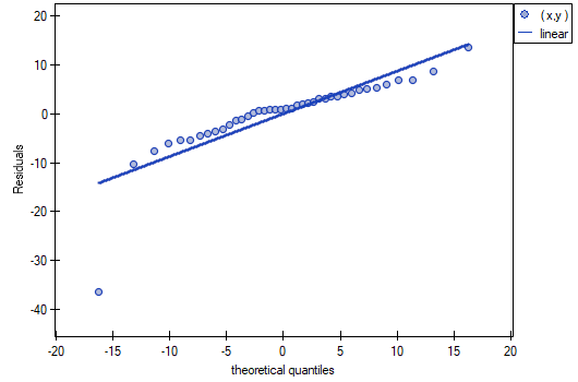
- Normality of the distribution of model residuals – we check this assumption visually using a Q-Q plot of the normal distribution. A large difference between the distribution of the residuals and the normal distribution may disturb the assessment of the significance of the coefficients of the individual variables in the model.
- Homoscedasticity (constancy of variance) – to check whether there are areas where the variance of the model residuals is increased or decreased, we use plots of the residuals (or the square of the residuals) against the predicted and observed values.
- Autocorrelation of model residuals – for the constructed model to be considered correct, the residual values should not be correlated with each other. This assumption can be checked using the Durbin-Watson test statistic.
Performing and interpreting the analysis
Example 1. (publisher.pqs file)
A certain book publisher wanted to find out what effect variables such as: production costs, advertising costs, direct promotion costs, the sum of discounts offered, and the author's popularity have on gross profit from sales. To do this, they analysed 40 titles published over the previous year (training set). An excerpt of the data is shown below:
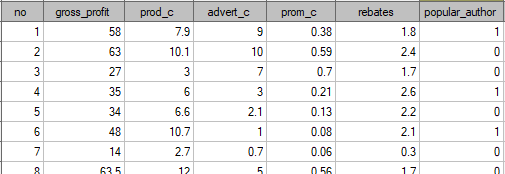
The first five variables are expressed in thousands of dollars – these are therefore variables collected on an interval scale. The last variable, author's popularity, is a dichotomous variable, where 1 means a known author and 0 means an unknown author. Based on the knowledge gained, the publisher plans to predict the gross profit from the next book published by a known author. The costs they intend to incur are: production costs \(\approx 11\), advertising costs \(\approx 13\), direct promotion costs \(\approx 0.5\), sum of discounts offered \(\approx 0.5\).
We build a multiple linear regression model for the training set, choosing: gross profit – as the dependent variable \(Y\), production costs, advertising costs, direct promotion costs, sum of discounts offered, author's popularity – as the independent variables \(X_1, X_2, X_3, X_4, X_5\). As a result, the coefficients of the regression equation will be calculated, along with measures allowing the quality of the model to be assessed.
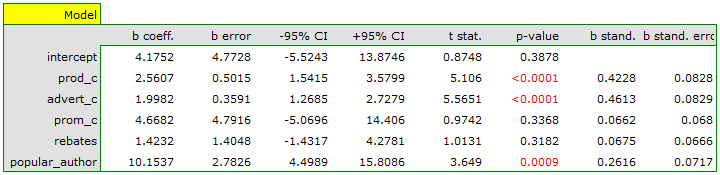
Based on the estimated value of the coefficient \(b\), the relationship between gross profit and all the independent variables can be described by the equation:
The coefficients obtained are interpreted as follows:
- if production costs increase by 1 thousand dollars, gross profit will increase by about 2.56 thousand dollars, assuming the other variables do not change;
- if advertising costs increase by 1 thousand dollars, gross profit will increase by about 2 thousand dollars, assuming the other variables do not change;
- if direct promotion costs increase by 1 thousand dollars, gross profit will increase by about 4.67 thousand dollars, assuming the other variables do not change;
- if the sum of discounts offered increases by 1 thousand dollars, gross profit will increase by about 1.42 thousand dollars, assuming the other variables do not change;
if the book was written by a known author (marked as 1), we assume the value 1 for author's popularity in the model and obtain the equation:
\[ profit_{gross}=14.33+2.56(c_{prod})+2(c_{adv})+4.67(c_{prom})+1.42(discounts) \]If, on the other hand, the book was written by an unknown author (marked as 0), we assume the value 0 for author's popularity in the model and obtain the equation:
\[ profit_{gross}=4.18+2.56(c_{prod})+2(c_{adv})+4.67(c_{prom})+1.42(discounts) \]
The result of the \(t\)-test obtained for each variable shows that only production costs, advertising costs, and author's popularity have a significant effect on the profit obtained. At the same time, the standardized coefficients \(b\) are largest for these variables.
Based on the interpretation of the results so far, we can suspect that some of the variables have no significant effect on profit and may be redundant. For the model to be well formulated, the interval-scaled independent variables should be strongly correlated with the dependent variable and relatively weakly correlated with each other. We can check this by calculating the correlation matrix and the covariance matrix:
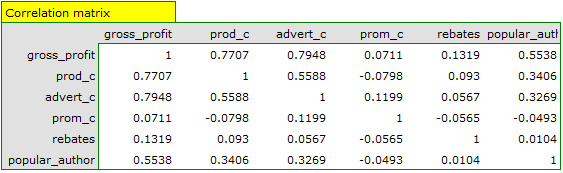
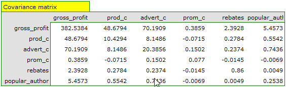
The most coherent information, allowing us to find those variables in the model that are redundant, is given by the analysis of partial and semi-partial correlation and redundancy:
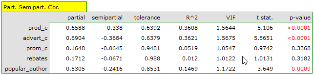
The values of the partial and semi-partial correlation coefficients indicate that direct promotion costs and the sum of discounts offered make the smallest contribution to the constructed model. However, these are the variables least correlated with the others in the model, as indicated by the low value of \(R^2\) and the high tolerance value. Ultimately, from a statistical point of view, models without these variables would not be worse than the current model (see the result of the \(t\)-test for comparing models). It is up to the researcher's decision whether to keep this model or build a new one without direct promotion costs and the sum of discounts offered. We will keep the current model.
Finally, we will perform an analysis of the residuals. An excerpt of this analysis is shown below:
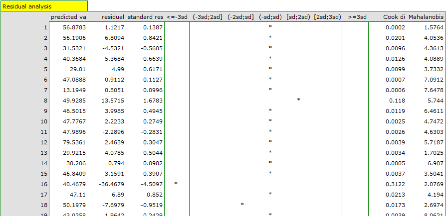
We can see that one of the model residuals is an outlier – it is more than 3 standard deviations from the mean value. This is observation number 16. We can easily find this observation by plotting a graph of residuals against the observed or predicted values of the variable \(Y\).
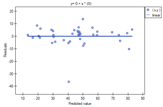
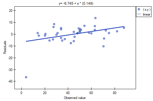
This outlying point disturbs the assumption of homoscedasticity – it would be satisfied (i.e. the variance of the residuals shown on the \(Y\) axis would be similar as we move along the \(X\) axis) if we rejected this point. Additionally, the distribution of the residuals deviates slightly from the normal distribution (the \(p\) value of the Lilliefors test is \(p=0.016415\)):
Looking more closely at the outlying point (position 16 in the task data), we see that this is the only book for which the costs are higher than the gross profit (gross profit = 4 thousand dollars, sum of costs = (8+6+0.33+1.6) = 15.93 thousand dollars).
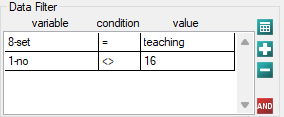
The resulting model can be improved by removing the outlier from it. This requires running the analysis again with a filter enabled that excludes the outlier.
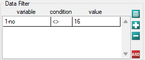
As a result, we obtain a very similar model, but with a smaller error and a better fit:
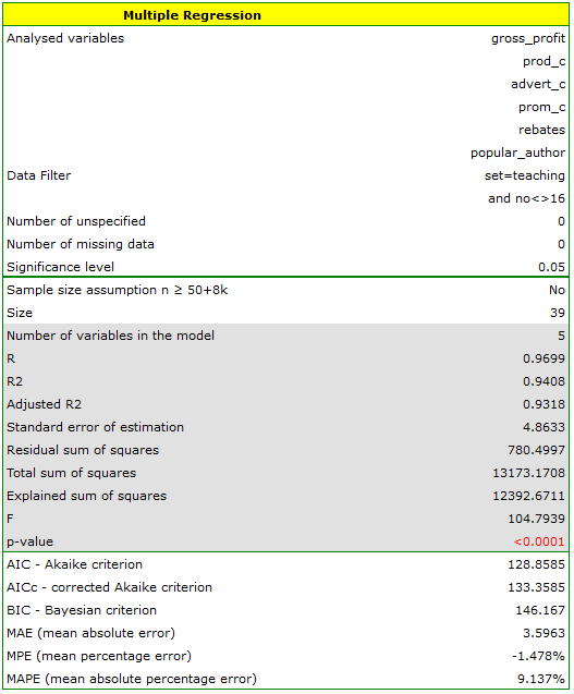
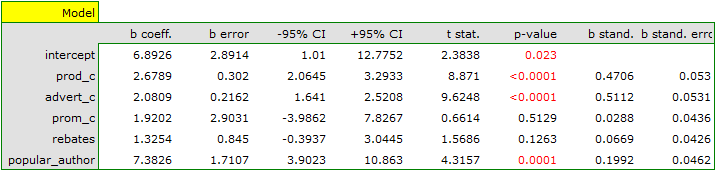
We will finally use the constructed model for prediction. Based on the predicted expenses in the amount of: production costs \(\approx 11\) thousand dollars, advertising costs \(\approx 13\) thousand dollars, direct promotion costs \(\approx 0.5\) thousand dollars, sum of discounts offered \(\approx 0.5\) thousand dollars, and the fact that the author is known (author's popularity \(\approx 1\)), we calculate the predicted gross profit together with the confidence interval:
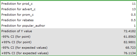
The predicted profit is 72 thousand dollars.
Finally, it should be noted that this is only a preliminary model. In an actual study, more data would need to be collected, since the number of variables in the model is too small relative to the number of books evaluated, i.e. \(n<50+8k\).
\(t\)-test for the significance of individual variables
Hypotheses:
\(\begin{array}{cc} \mathcal{H}_0: & \beta_i=0,\\ \mathcal{H}_1: & \beta_i\ne 0. \end{array}\)
Formulas: the test statistic is defined by:
The test statistic has the \(t\)-Student distribution with \(n-k\) degrees of freedom.
The \(p\) value, determined on the basis of the test statistic, is compared with the significance level \(\alpha\): if \(p \le \alpha\), we reject \(\mathcal{H}_0\) in favor of \(\mathcal{H}_1\); if \(p > \alpha\), there is no reason to reject \(\mathcal{H}_0\).
Standard error of estimation
Multiple coefficient of determination
In its determination, we use the following equality:
where:
\(T_{SS}\) – the total sum of squares,
\(E_{SS}\) – the sum of squares explained by the model,
\(R_{SS}\) – the residual sum of squares.
The coefficient of determination is calculated from the formula:
The adjusted value of this parameter:
Information criteria
\(AIC\), \(AICc\), and \(BIC\) represent a kind of trade-off between goodness of fit and complexity. The second term in the sum in the formulas for the information criteria (the so-called loss or penalty function) measures the simplicity of the model – it depends on the number of variables in the model (\(k\)) and the sample size (\(n\)).
Akaike information criterion (Akaike information criterion)
where the constant can be omitted, since it is the same in each of the compared models. This is an asymptotic criterion – suitable for large samples, i.e. when \(\frac{n}{k+2}>40\). For small samples, it tends to favour models with a large number of variables.
Example of interpreting an AIC comparison
Suppose we determined AIC for three models: \(AIC_1\)=100, \(AIC_2\)=101.4, \(AIC_3\)=110. We can then determine the relative likelihood of each model, calculated relative to another model, usually the one with the smallest AIC value, using the formula: \(e^{(AIC_{min} - AIC_i)/2}\). Comparing model 2 to model 1, the probability that it minimizes information loss is about half the probability that model 1 does so (exactly \(\exp((100-101.4)/2) = 0.497\)). Comparing model 3 to model 1, this probability is only a small fraction of the probability for model 1 (exactly \(\exp((100-110)/2) = 0.007\)).
Corrected Akaike information criterion
The Akaike criterion correction relates to sample size, which is why this measure is also recommended for small samples.
Bayesian information criterion (Schwarz criterion)
Like the corrected Akaike criterion, BIC takes sample size into account.
Error analysis for ex post forecasts
MAE (mean absolute error) – the accuracy of the forecast, as determined by MAE, tells us how much, on average, the actual realisations of the dependent variable deviate (in absolute value) from the forecasts.
MPE (mean percentage error) – indicates what average percentage of the realisations of the dependent variable the forecast errors represent.
MAPE (mean absolute percentage error) – indicates the average size of forecast errors, expressed as a percentage of the actual values of the dependent variable. MAPE allows the accuracy of forecasts obtained from different models to be compared.
F-test – statistical significance of all variables in the model
This test verifies 3 equivalent hypotheses at the same time:
Formulas: the test statistic is defined by:
where:
\(\displaystyle E_{MS}=\frac{E_{SS}}{df_{E}}\) – the mean square explained by the model,
\(\displaystyle R_{MS}=\frac{R_{SS}}{df_{R}}\) – the residual mean square,
\(df_E=k\), \(df_R=n-(k+1)\) – the corresponding degrees of freedom.
This statistic has the F Snedecor distribution with \(df_E\) and \(df_R\) degrees of freedom.
The \(p\) value, determined on the basis of the test statistic, is compared with the significance level \(\alpha\): if \(p \le \alpha\), we reject \(\mathcal{H}_0\) in favor of \(\mathcal{H}_1\); if \(p > \alpha\), there is no reason to reject \(\mathcal{H}_0\).
Cook's distance and Mahalanobis distance – described above in the practical section.
Autocorrelation of residuals – the Durbin-Watson statistic
Interpretation: to test for positive autocorrelation at the significance level \(\alpha\), we check the position of the statistic \(d\) relative to the upper (\(d_{U,\alpha}\)) and lower (\(d_{L,\alpha}\)) critical value:
- if \(d <d_{L,\alpha}\) – the errors are positively correlated;
- if \(d> d_{U,\alpha}\) – the errors are not positively correlated;
- if \(d_{L,\alpha}<d <d_{U,\alpha}\) – the test result is inconclusive.
To test for negative autocorrelation at the significance level \(\alpha\), we check the position of the value \(4-d\) relative to the upper and lower critical value:
- if \(4-d <d_{L,\alpha}\) – the errors are negatively correlated;
- if \(4-d> d_{U,\alpha}\) – the errors are not negatively correlated;
- if \(d_{L,\alpha}<4-d <d_{U,\alpha}\) – the test result is inconclusive.