The intraclass correlation coefficient and a test to examine its significance

When to use:

The intraclass correlation coefficient (ICC) is used when the measurement of the variable studied is made by several “raters” (\(k\geq2\)). It measures the strength of interrater reliability, i.e. the degree to which their ratings agree. Since it can be determined in several different situations, there are several variants of it, depending on the model and the type of agreement.

Assumptions

measurement on an interval scale,
the normal distribution for all variables that are the differences of measurement pairs (or normality of the analysed variable for each measurement),
for model 1 – an independent model, for model 2 / 3 – a dependent model.

Definitions of measures

Depending on the variability present in the data, two main research models and two types of agreement are distinguished.

Model 1 – for each of the \(n\) randomly selected objects rated, a set of \(k\) raters is randomly selected from the population of raters, and a different set of raters may be drawn for each object. The ICC coefficient is then determined using the ANOVA for independent groups random model. ICC(1,1) answers the question of the reliability of a single rater's ratings, and ICC(1,k) the reliability of a result that is the average of \(k\) raters' ratings.

Model 2 – a set of \(k\) raters is randomly selected from the population of raters, and each of them rates all \(n\) random objects. The ICC coefficient is then determined using the ANOVA for dependent groups random model. Depending on the type of agreement sought, we can estimate:

absolute agreement – raters are in absolute agreement if they give exactly the same ratings, e.g. perfectly agreeing would be ratings given by a pair of raters (2,2), (5,5), (8,8);
consistency – raters may use different ranges of values, but apart from this shift there should be no differences, in order to keep the verdict consistent, e.g. perfectly consistent would be ratings given by a pair of raters (2,5), (5,8), (8,11).

As in model 1, ICC(2,1) answers the question of the reliability of a single rater's ratings, and ICC(2,k) the reliability of a result that is the average of \(k\) raters' ratings (the formulas differ depending on the type of agreement chosen).

Note! Sometimes it is necessary to consider model 3[154], i.e. a set of \(k\) raters is selected and each of them rates all \(n\) random objects, but the agreement result applies only to these particular \(k\) raters. The ICC coefficient is then determined in a mixed model (since the randomness concerns only the objects, not the raters). Since we ignore the variability concerning the raters, we examine consistency (rather than absolute agreement), and the coefficients from the second model apply: ICC(2,1) and ICC(2,k), since they are identical to the coefficients ICC(3,1) and ICC(3,k) that would be desired in this case, under the assumption of no interaction between objects and raters.

Interpretation – the value \(ICC\in\langle-1;1\rangle\) is interpreted as follows:

\(ICC\approx1\) means strong agreement in the rating of individual objects by the raters, which is reflected in high variance between objects (a significant difference in means among the \(n\) objects) and low variance between raters' ratings (a small difference in the mean ratings determined for the \(k\) raters);
\(ICC\approx-1\) – a negative intraclass correlation coefficient is treated in the same way as \(ICC\approx0\);
\(ICC\approx0\) means no agreement in the rating of individual objects by the raters, which is reflected in low variance between objects (a small difference in means among the \(n\) objects) and high variance between raters' ratings (a significant difference in the mean ratings determined for the \(k\) raters).

How to set up the analysis

Statistics \(\to\) Parametric tests \(\to\) ICC – Intraclass Correlation Coefficient (or via the Wizard).

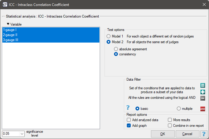
Performing and interpreting the analysis

Example 1. (sound intensity.pqs file)
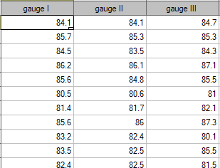
In order to effectively protect the hearing of workers at a workplace, it is first necessary to reliably estimate the sound intensity at the various locations where people are present. At one company, it was decided to conduct an experiment before choosing a sound-intensity meter (sonograph). Sound-intensity measurements were made at 42 randomly selected measurement points on the company premises, using 3 randomly drawn analogue sonographs and 3 randomly selected digital sonographs. An excerpt of the measurements collected is shown in the table below.

To find out which type of instrument (analogue or digital) better accomplishes the task at hand, the ICC coefficient should be determined in model 2, examining absolute agreement. The type of meter with the higher ICC value will provide more reliable measurements, and will therefore be used at the company site in the future.

The analysis performed for the analogue meters shows significant agreement of the measurements.

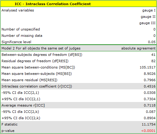
\(p<0.000001\) for the analogue meters (statistically significant, \(\alpha=0.05\))

The reliability of the measurement made with a single analogue meter is \(ICC(2,1)=0.45\), and the reliability of a measurement that is the average of the three analogue meters is \(ICC(2,k)=0.71\).

However, the lower limit of the 95% confidence interval for these coefficients is worryingly low. A similar analysis performed for the digital meters gave better results.

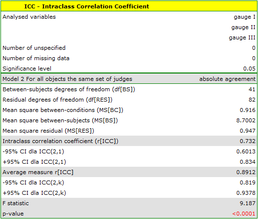
\(p<0.000001\) for the digital meters (statistically significant, \(\alpha=0.05\))

The ICC coefficients and their confidence intervals are much higher than for the analogue meters: \(ICC(2,1)=0.73\), \(ICC(2,k)=0.89\).

Digital meters will therefore be used at the company site from now on. The agreement of the results obtained for the digital meters is shown on a scatter plot, where each measurement point is described by the sound-intensity value obtained for each meter.

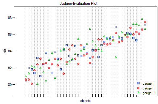
By plotting the previously sorted data according to the mean sound-intensity value, we can check whether the degree of agreement increases or decreases as sound intensity increases. For our data, slightly higher agreement (closeness of the points on the graph) is observed at high sound-intensity values. Similarly, the agreement of the results obtained can be observed on Bland-Altman plots [8][23] constructed separately for each pair of meters. The plot for meter I and meter II is shown below.

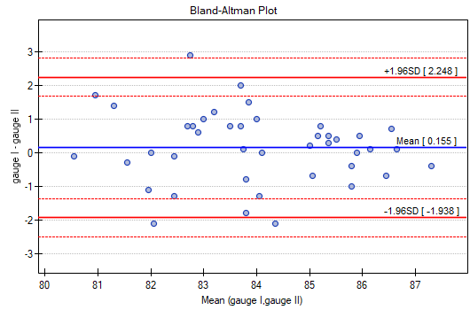
Here too, we observe higher agreement (points concentrated close to the horizontal axis \(y=0\)) for higher sound-intensity values.

Note! If the researcher were not concerned with estimating the actual sound-intensity value at the company site, but instead wanted to identify locations where this level is higher than elsewhere, or to check whether the noise level changes over time, then model 2 examining consistency would be a sufficient model.

FOR THOSE INTERESTED

Model 1 – formulas:
ICC(1,1):

\[ ICC(1,1)=\frac{MS_{WG}-MS_{BG}}{MS_{WG}+(k-1)MS_{BG}}. \]

ICC(1,k):

\[ICC(1,k)=\frac{MS_{WG}-MS_{BG}}{MS_{WG}},\]

where:
\(MS_{WG}\) – mean square within-groups,
\(MS_{BG}\) – mean square between-objects.

Model 2 – absolute agreement – formulas:
ICC(2,1):

\[ ICC(2,1)=\frac{MS_{BS}-MS_{res}}{MS_{BS}+(k-1)MS_{res}+\frac{k}{n}(MS_{BC}-MS_{res})}. \]

ICC(2,k):

\[ICC(2,k)=\frac{MS_{BS}-MS_{res}}{MS_{BS}+(MS_{BC}-MS_{res})/n},\]

where:
\(MS_{BC}\) – mean square between-raters,
\(MS_{BS}\) – mean square between-objects,
\(MS_{res}\) – mean square residual.

Model 2 – consistency – formulas:
ICC(2,1):

\[ ICC(2,1)=\frac{MS_{BS}-MS_{res}}{MS_{BS}+(k-1)MS_{res}}, \]

ICC(2,k):

\[ICC(2,k)=\frac{MS_{BS}-MS_{res}}{MS_{BS}},\]

where:
\(MS_{BS}\) – mean square between-objects,
\(MS_{res}\) – mean square residual.

The F-test for the significance of the intraclass correlation coefficient
Hypotheses:

\(\begin{array}{cl} \mathcal{H}_0: & ICC=0 \\ \mathcal{H}_1: & ICC\neq 0 \quad(ICC=1) \end{array}\)

Formulas:
The test statistic is defined by:

\[ F=\frac{MS_{BS}}{MS_{res}} \textrm{ -- in the dependent model,} \]

\[ F=\frac{MS_{WG}}{MS_{BG}} \textrm{ -- in the independent model.} \]

The test statistic has the F Snedecor distribution with the number of degrees of freedom defined in the model.

The \(p\) value, determined on the basis of the test statistic, is compared with the significance level \(\alpha\): if \(p \le \alpha\), we reject \(\mathcal{H}_0\) in favor of \(\mathcal{H}_1\); if \(p > \alpha\), there is no reason to reject \(\mathcal{H}_0\).