 PQStat
 Introduction: dependent data, fixed effects and random effects
Why mixed models
The classical regressions available in the program – multiple regression, logistic regression and Cox regression – assume that all observations are independent of one another. In many studies this assumption does not hold, because observations naturally fall into groups:
- repeated measurements – the same patient examined several times (before treatment, after a week, after a month), the same person tested on consecutive days;
- clustered data – patients treated in the same centre, pupils from the same class, animals from one litter or herd;
- hierarchical data – measurements of a patient, patients within a centre, centres within a region (several levels of nesting);
- recurrent events and paired objects – successive infections of the same patient, the two eyes of the same person.
Observations from the same group are more alike than observations from different groups: a patient with high blood pressure usually has high pressure at every visit, and a centre with poorer outcomes has poorer outcomes for most of its patients. If we ignore this dependence and fit an ordinary regression, the program treats e.g. 10 measurements of one patient as 10 independent people. The consequences are twofold:
- standard errors are underestimated and \(p\)-values are too small – we declare effects significant too easily (so-called pseudoreplication);
- we do not know what share of the variability comes from differences between groups (people, centres) and what share from variability within groups, although this is often the most interesting information in the study.
A mixed model solves both problems: it accounts for the group structure when computing errors, and it explicitly estimates how much the groups differ from one another.
Fixed effects and random effects
The name „mixed model” comes from the fact that the model contains two kinds of effects:
- fixed effects – the ordinary regression coefficients \(\beta_0, \beta_1, \ldots\) of the independent variables. They describe the population as a whole and are interpreted exactly as in classical regression: by how much \(Y\) changes when \(X\) increases by one unit;
- random effects – deviations of individual groups from what the fixed effects predict. We are not interested in the individual values of these deviations for each group, but in their variance, i.e. a measure of how much the groups differ. We assume that the groups in the study are a random sample from a larger population of groups (patients, centres), and that their effects are normally distributed with mean 0.
The simplest random effect is a random intercept: each group has its own level of \(Y\), shifted relative to the population level. If, in addition, the effect of some variable (most often time) differs between groups, we introduce a random slope of that variable. The figure below shows the difference: on the left the groups have different levels but the same trend; on the right they also differ in the rate of change.
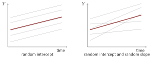
Thick line – fixed effects (population); thin lines – individual groups.
The three mixed models in the program
Each classical regression has a mixed counterpart in the program. The choice depends solely on the type of the dependent variable:
| Dependent variable | Classical model | Mixed model | Random effects |
| continuous | multiple regression | mixed multiple regression | intercept, slopes |
| binary (0/1) | logistic regression | mixed logistic regression | intercept, slopes |
| time and status | Cox PH regression | Cox regression with random effect | group frailty |
Mixed multiple regression replaces repeated measures ANOVA when measurements are incomplete, unevenly spaced in time, or when continuous variables are to be included in the model. Mixed logistic regression plays the same role with respect to Cochran's Q ANOVA. Cox regression with random effect is the counterpart of Cox regression for patients from many centres or for recurrent events.
Data preparation: long format
All three analyses require data in long format: each row of the sheet is one observation (one measurement), and a separate column – the grouping variable (ID) – says which group the observation belongs to. The grouping variable can be a number, text or date; the program treats it purely as a label. Groups may have different numbers of observations, and missing data are removed row by row, not group by group.
|
| ||||||||||||||||||||||||||||||||||||||||||||
Data stored in wide format (successive measurements in successive columns, as in repeated measures ANOVA) must be rearranged into long format before the analysis: the measurement columns are copied one below another into a common column of values, next to it we enter the object identifier (repeated as many times as there are measurements) and the number or time of the measurement. This rearrangement is performed automatically by the command Data\(\to\)Reshape: wide \(\to\) long... (see reshaping data between the wide and the long format); the reverse command Reshape: long \(\to\) wide... returns to the wide layout. The commands Create raw data and Create table serve a different purpose – they convert a contingency table (counts) into raw data and back.
What to read in the report and in what order
The reports of the three models share a common layout. Recommended reading order:
- Convergence and singular fit. If the algorithm did not converge, or the report flags a singular fit (a random-effect variance practically equal to zero, or a random-effects correlation equal to \(\pm1\)), the remaining numbers are unreliable. The model should be simplified: remove a random slope, choose the independent covariance, or reduce the number of variables.
- ICC from the null model. The intraclass correlation coefficient says what share of the total variability of \(Y\) lies between groups. An ICC close to 0 means that observations within a group are almost independent; an ICC of 0.4 means that 40% of the variability is due to differences between groups, and two observations from the same group are correlated at 0.4. A small ICC is not, however, a reason to abandon the mixed model if the study design is hierarchical – the mixed model remains the correct method, and ordinary regression does not.
- Random effects test. The likelihood ratio (LR) test compares the mixed model with a model without random effects. The null hypothesis (variance equal to 0) lies on the boundary of the admissible values, so the program corrects the \(p\)-value (a mixture of \(\chi^2\) distributions; in the simplest case the \(p\)-value is halved) and says so in the report.
- Random effects. The standard deviation of the random intercept is expressed in units of \(Y\) (in logistic and Cox regression – on the logit or log-hazard scale) and says how far a typical group departs from the mean. The standard deviation of a random slope says how much the groups differ in their rate of change.
- Fixed effects. Read as in classical regression, with one difference: in logistic and Cox regression the odds ratio and hazard ratio are conditional – they describe the effect of a variable „within the same group” (for the same patient, the same centre). In absolute value they are larger than the population OR and HR from ordinary regression, which averages over groups, and the two should not be compared directly.
- Group random effects (BLUP). Predicted deviations of the individual groups. They serve to point out atypical groups (a patient with an outlying trajectory, a centre with a higher risk), not to test significance. The „caterpillar” plot (groups ordered by effect, with intervals) shows them most clearly.
How many groups are needed
The variance of a random effect is estimated from the number of groups, not the number of observations. The program requires at least 3 groups, but with fewer than 10 groups it warns that the variance estimate is uncertain. In practice reliable estimates begin at ten to several dozen groups, and each random slope raises these requirements. With 3–5 centres it is more sensible to treat the centre as a dummy variable (fixed effect) than as a random effect.
Limitations
Mixed models are not included in Test summaries or in the Wizard. Two levels of nesting (e.g. patient within centre) and the AR(1) and exchangeable residual correlation structures are available in mixed multiple regression; in Cox regression with random effect only a random intercept (gamma frailty) is available.