 PQStat
 Mixed multiple regression (linear mixed model)
When to use:
Mixed multiple regression (linear mixed model, LMM) extends multiple linear regression to data in which observations are not independent but form groups: repeated measurements of the same patient, patients treated in the same centre, pupils from one class, animals from one litter (see the introduction to mixed models). Observations from the same group are more alike than observations from different groups. Ordinary regression ignores this dependence, which underestimates the standard errors of the coefficients and overstates significance. A mixed model splits the variability of the dependent variable into a between-group part and a within-group part, and every coefficient receives a proper error.
The model contains two kinds of effects:
- fixed effects – the ordinary regression coefficients \(\beta_0,\beta_1,\ldots,\beta_k\) describing the population,
- random effects – deviations of individual groups from the population: a random intercept (each group has its own level of \(Y\)) and optionally random slopes (the effect of a chosen variable \(X\) differs between groups).
A model with a random intercept and a random slope of \(X_1\) has the form:
where:
\(Y_{ij}\) – the \(i\)-th observation in group \(j\),
\(\beta_0,\beta_1,\ldots,\beta_k\) – fixed effects,
\(u_{0j}\) – the random intercept of group \(j\), \(u_{1j}\) – the random slope of group \(j\); \((u_{0j},u_{1j})\) are assumed normal with mean 0 and covariance matrix \(\Sigma\) (variances \(\tau_0^2\), \(\tau_1^2\) and correlation \(\rho_{01}\)),
\(\epsilon_{ij}\) – the residual, normal with mean 0 and variance \(\sigma^2\).
For group \(j\) the model thus describes its own straight line: its intercept is \(\beta_0+u_{0j}\) and its slope \(\beta_1+u_{1j}\). The fixed effects describe the line of the „average” group, and the random-effect variances – how widely the lines of the individual groups are scattered around it.
This model replaces repeated measures ANOVA when the repeated measurements are incomplete or unevenly spaced in time, when the number of measurements differs between subjects, or when, besides the repeated factor, the model is to contain continuous variables (e.g. age, dose) or variables describing the group (e.g. sex, centre).
Assumptions
- the dependent variable \(Y\) is measured on an interval scale,
- a linear relationship between the dependent variable and the independent variables,
- random effects and residuals are normally distributed; residuals have constant variance,
- groups are independent of one another – dependence occurs only within groups,
- a sufficient number of groups – at least 3, and usually a dozen or more for a reliable estimate of the random-effect variances,
- missing data are random (the model does not require complete or balanced measurements).
Definitions of measures
Random-effect variances – \(\tau_0^2\) (random intercept) says how much the groups differ in the level of \(Y\); \(\tau_1^2\) (random slope) – how much they differ in the effect of \(X_1\). Their square roots, the standard deviations, are easier to read because they are expressed in units of \(Y\) (or \(Y\) per unit of \(X_1\)): a typical group departs from the population by about one standard deviation, and about 95% of groups fall within \(\pm2\) deviations.
Random-effects correlation \(\rho_{01}\) – the relationship between a group's level and its slope. A negative correlation means that groups starting higher change more slowly. Note: its value depends on where the zero of \(X_1\) lies – the intercept is the level at \(X_1=0\). When \(X_1\) is e.g. age 8–14 years, it is worth centring it (subtracting the middle value) so that the correlation describes the level in the middle of the range rather than a hypothetical level at age 0.
Intraclass correlation coefficient (ICC) – computed from the null model (no independent variables, only a random intercept):
where \(\tau^2\) is the between-group variance and \(\sigma^2\) the within-group (residual) variance. The ICC is the share of between-group variability in the total variability and, at the same time, the correlation of two observations from the same group. Its confidence interval is approximate (delta method).
Marginal and conditional \(R^2\) (Nakagawa and Schielzeth 2013[191]) – the marginal \(R^2\) is the share of variance explained by the fixed effects alone, the conditional \(R^2\) – by the fixed and random effects together. Their difference says how much variability is „explained” by group membership.
LR test of random effects – a likelihood ratio test comparing the model with and without a given random effect. The null hypothesis (variance equal to 0) lies on the boundary of the parameter space, so the \(p\)-value from the \(\chi^2\) distribution is corrected (a mixture of distributions; for a single parameter the \(p\)-value is halved). The program always computes this test by ML, regardless of the estimation method chosen for the main model.
Group random effects (BLUP) – predicted values of \(u_{0j}\), \(u_{1j}\) for each group (best linear unbiased predictor). They are „shrunk” towards zero: a group with few observations or a large scatter receives an effect closer to 0 than the plain mean of its observations would suggest. They serve to identify atypical groups and to predict for a specific group, not to test significance.
Singular fit – a situation in which the estimated variance of some random effect is practically 0, or the random-effects correlation equals \(\pm1\). The model is then too complex for the data and should be simplified (remove the random slope or choose the independent covariance).
Satterthwaite degrees of freedom – in a mixed model there is no single simple number of degrees of freedom for the test of a fixed effect. A variable describing the group (e.g. the patient's sex) effectively has as many independent observations as there are groups, while a variable varying within groups has more. The Satterthwaite method assigns each coefficient its own, usually non-integer, degrees of freedom, so that the \(t\)-test is reliable even with few groups.
Residual structure within group – by default the residuals \(\epsilon_{ij}\) are independent and all within-group correlation comes from the random effects. For measurements over time one may additionally assume that residuals of neighbouring measurements are correlated: AR(1) (the correlation \(\rho\) decays exponentially with the distance in the row order of the group: \(\rho, \rho^2, \rho^3, \ldots\)) or exchangeable (CS) (equal correlation of all pairs of residuals within the group).
Level 2 – a second, superordinate level of grouping, e.g. patient (level 1) nested within centre (level 2). The model then receives two random intercepts, and the report – a variance and an ICC separately for each level.
How to set up the analysis
Statistics \(\to\) Mixed models \(\to\) Mixed multiple regression.
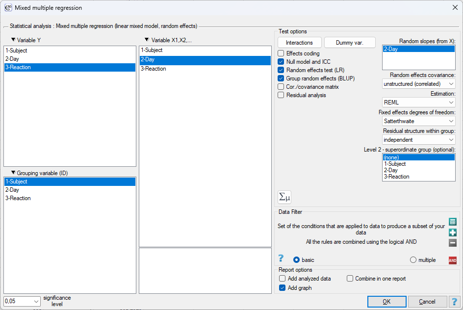
The analysis window has the layout known from multiple regression. In its left part we indicate the variables:
- Dependent variable Y – the continuous variable to be explained,
- Grouping variable (ID) – the column identifying the group (patient, centre, litter); numeric or text,
- Independent variables X1, X2, … – predictors; dummy variables and interactions are prepared with the Dummy variables and Interactions buttons as in multiple regression (chapter Preparing variables for analysis in multidimensional models).
The right part of the window contains the mixed-model options. Below we describe what each of them changes.
Random effects
- Random slopes (from X) – the list is filled with the variables chosen as \(X\). Selecting a variable means that its effect is to differ between groups (e.g. the rate of change over time differs for each patient). The random intercept is always in the model and does not need to be selected. A variable with a random slope must vary within groups; a variable constant within a group (e.g. the patient's sex) cannot have a random slope – the program will report an error. Each random slope adds a variance and (with the unstructured covariance) correlations to the model, so it requires more groups; it is sensible to start with a single slope, most often for time.
- Random effects covariance – unstructured (correlated) also estimates the correlation between the random intercept and the slope (and between slopes); independent sets these correlations to 0. The independent variant has fewer parameters, is more stable with few groups, and is recommended when the correlation in the full model comes out close to 0 or \(\pm1\) (singular fit). Without random slopes the option has no effect.
Estimation
- Estimation – REML (restricted maximum likelihood, default) gives unbiased variance estimates and is recommended for the final model; ML (maximum likelihood) slightly underestimates the variances, but only the ML likelihood allows models differing in fixed effects to be compared with information criteria. The choice of method does not noticeably change the fixed-effect coefficients, but it does change the random-effect variances, their errors and the values of \(-2LL\), AIC, BIC. Rule: variable selection – ML, reporting the model – REML.
- Fixed effects degrees of freedom – Satterthwaite (default) assigns each coefficient its own degrees of freedom and a \(t\)-test; always recommended, especially with few groups. Wald z test treats the statistic as in a large sample (normal distribution, no degrees of freedom); it gives smaller \(p\)-values and is appropriate only with many groups.
- Residual structure within group – independent (default), AR(1) (row order) or exchangeable (CS). AR(1) requires the rows of each group to be ordered in time in the sheet and roughly equally spaced. The parameter \(\rho\) appears in the report. Exchangeable together with a random intercept is not identifiable (both describe the same constant within-group correlation), so it makes sense mainly as a comparison with the AR(1) model.
- Level 2 – superordinate group (optional) – the column indicating the higher-level group in which the grouping variable is nested (e.g. centre for patients). It adds a level-2 random intercept and, in the report, a separate variance, ICC and BLUP table for that level.
Report elements
- Null model and ICC – a model without independent variables is additionally fitted and the ICC with its confidence interval is derived from it; worth leaving on, because the ICC is the first number to look at.
- Random effects test (LR) – likelihood ratio tests for each random component separately and for all of them jointly (mixed model versus ordinary multiple regression). Lengthens the computation, because additional models must be fitted.
- Group random effects (BLUP) – adds a table of the predicted effects of each group with errors; with hundreds of groups the table is long, and the same values are shown by the caterpillar plot.
- Cor./covariance matrix – correlation and covariance matrices of the fixed-effect estimates.
- Residual analysis – fitted values (conditional and population), residuals and standardized residuals for every observation.
- Add graphs – the caterpillar plot of group random effects and (with a random slope) group trajectories against the population line.
The remaining elements of the window (significance level, data filter, merging reports) work as in other analyses.
Results and interpretation
Counts – number of observations, number of groups and the minimum, median and maximum number of observations per group. With fewer than ten groups the report warns that the random-effect variance estimates are uncertain.
Estimation – method (REML/ML), number of iterations, information on convergence and on singular fit. Non-convergence or a singular fit means the model must be simplified before the remaining results are interpreted.
Model fit – log-likelihood, \(-2LL\), the information criteria AIC, AICc and BIC (the smaller, the better the model) and the marginal and conditional \(R^2\). Information criteria may only be compared between models fitted by the same method; models differing in fixed effects – only under ML.
LR test of random effects (vs multiple regression, ML) – whether accounting for the group structure is needed at all. A significant result means that ordinary multiple regression is not valid for these data. A non-significant result with a hierarchical design does not, however, exempt one from using the mixed model.
Null model – between-group variance \(\tau^2\), residual variance \(\sigma^2\) and the ICC with its confidence interval.
Fixed effects (conditional) – coefficient \(b\), its error, confidence interval, the \(t\) statistic with Satterthwaite degrees of freedom (may be non-integer) or the \(z\) statistic, and the \(p\)-value. Interpretation as in multiple regression: \(b\) is the change of \(Y\) per unit of \(X\) with the other variables held fixed, within the same group. The degrees of freedom hint at the level at which a variable „operates”: a number close to the number of groups indicates a variable describing groups, a number close to the number of observations – a variable varying within groups.
Random effects – for each component the variance and standard deviation. The columns LR \(\chi^2\), df and \(p\) contain the test of whether the component is needed (model with it versus without it, ML, boundary-corrected). The last row is the residual variance. With an AR(1) or CS structure the report gives the parameter \(\rho\), and with level 2 – the variance and ICC of that level.
Random effects correlations – with more than one component, the correlation matrix between the random intercept and the slopes. A value close to \(\pm1\) signals a singular fit.
Group random effects (BLUP) – the predicted deviation of each group from the population with its error (for the intercept and each random slope). The sum of the fixed effect and the BLUP gives the group's own coefficient. On the caterpillar plot, groups whose interval does not include zero clearly depart from the average.
Residual analysis – conditional fitted values (with the group's random effects, i.e. „for this patient”) and population fitted values (fixed effects only, i.e. „for the average patient”), residuals and standardized residuals; observations with \(|residual|\ge3\) are flagged as outliers.
Graphs – Group random effects (BLUP \(\pm\) error): groups ordered by the value of the effect, with an error interval and a zero line; a separate panel for the intercept and for each slope. Group trajectories: for a model with a random slope, thin lines fitted for the individual groups against the thick population line – the most vivid summary of repeated measurements.
Execution and interpretation
Example 1. (sleepDeprivation.pqs file)
In a study of the effect of sleep loss on psychomotor performance (Belenky et al. 2003[185]), 18 subjects were allowed only 3 hours of sleep per night for 10 consecutive days. Each day their average reaction time (in milliseconds) in a vigilance test was measured. The data are in long format: the column Subject identifies the person, Day is the day of deprivation (0–9) and Reaction – the reaction time. In total 180 observations, 10 per subject.
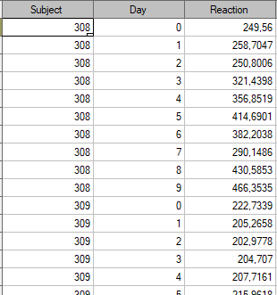
We want to answer three questions: (1) by how much does the reaction time lengthen with each day without sleep, (2) do people differ in their resistance to sleep loss, i.e. is the rate of deterioration the same for everyone, (3) which subjects react to deprivation most strongly.
If we fitted an ordinary multiple regression of reaction time on day, the program would treat the 180 measurements as 180 independent people, whereas in fact we have 18 people, each measured ten times. We therefore build a mixed model: Reaction as the dependent variable \(Y\), Subject as the grouping variable (ID), Day as the independent variable \(X_1\). Since we ask whether the rate of change differs between people, we select Day in the Random slopes list; we leave the covariance unstructured (correlated), the estimation REML, the degrees of freedom Satterthwaite. We switch on Null model and ICC, Random effects test (LR), Group random effects (BLUP) and Add graphs.
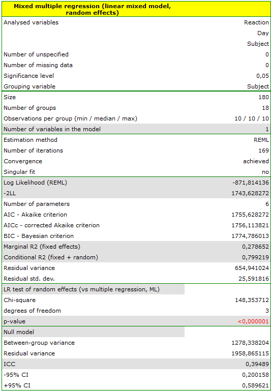
Step 1 – is the model properly fitted. The report gives 180 observations in 18 groups (10 observations per group), convergence achieved and no singular fit. We can read on.
Step 2 – how much variability lies between subjects (null model and ICC). In the null model the between-group variance is 1278.34 and the residual variance 1958.87, hence ICC \(=0.395\) (95% CI: 0.200–0.590). About 39% of the total variability of reaction time consists of stable differences between people (some have naturally faster reactions, others slower), and two measurements of the same person are correlated at 0.39. Far too much to treat the measurements as independent.
Step 3 – are random effects needed. The LR test of random effects against ordinary multiple regression gives \(\chi^2=148.35\), \(df=3\), \(p<0.000001\) – the group structure is indispensable.

Step 4 – fixed effects (answer to question 1). The intercept \(b_0=251.41\) ms (95% CI: 237.01–265.80) is the average reaction time on day 0, i.e. before deprivation. The coefficient of day \(b_1=10.47\) ms (95% CI: 7.21–13.73), \(t=6.77\), \(df=17.0\), \(p=0.000003\): each successive day without sleep lengthens the reaction time of an average person by about 10.5 ms. Note the degrees of freedom: they equal 17 (18 subjects minus 1), not 178, because it is 18 people who inform us about the rate of change, not 180 measurements. For comparison, ordinary multiple regression would give the same coefficient 10.47, but with an error of 0.80 instead of 1.55 – underestimated twofold.
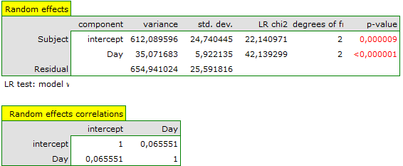
Step 5 – random effects (answer to question 2). The standard deviation of the random intercept is 24.74 ms: a typical person on day 0 differs from the average by about 25 ms, and most people (95%) fall within \(251\pm2\cdot25\), i.e. from about 200 to 300 ms. The standard deviation of the random slope is 5.92 ms/day: since the average rate is 10.5 ms/day, in some people the reaction lengthens by only 0–5 ms per day, in others by 15–20 ms. The LR test for the slope (\(\chi^2=42.14\), \(df=2\), \(p<0.000001\)) confirms that the rate of deterioration differs significantly between people. The correlation between the intercept and the slope is only 0.066 – how fast someone reacts at the start says nothing about how fast they will deteriorate. The residual variance 654.94 (standard deviation 25.59 ms) is the day-to-day variability of the same person's measurements, unexplained by their own line.
Marginal \(R^2=0.279\): the day of deprivation alone explains 28% of the variability of reaction time. Conditional \(R^2=0.799\): day together with the individual levels and slopes explains 80%. The difference (52 percentage points) is the variability attributed to differences between people.
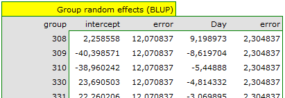
Step 6 – which subjects are atypical (answer to question 3). The BLUP table gives each subject's deviations from the population. Subject 308 has intercept \(+2.26\) (average start) and slope \(+9.20\): their reaction time grows by \(10.47+9.20\approx19.7\) ms per day, almost twice as fast as average – this is the person most sensitive to sleep loss. Subjects 309 and 310 start low (\(-40.4\) and \(-39.0\) ms respectively, i.e. they react fast) and have slopes \(-8.62\) and \(-5.45\): their reaction lengthens by only about 2 and 5 ms per day – they are almost immune to deprivation. The same information is shown by the graphs: the caterpillar plot (subjects ordered by effect, with an error interval) and the group trajectories (thin lines of the individual subjects against the thick population line).
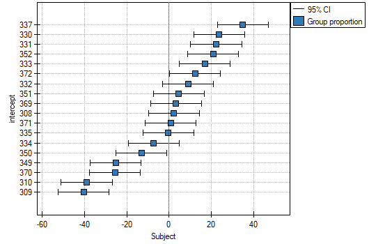
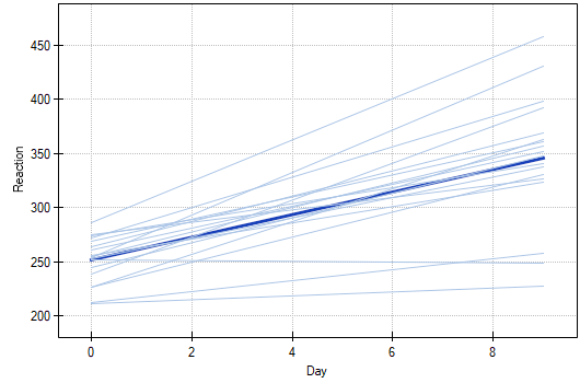
What other settings change. The same model fitted by ML gives identical fixed-effect coefficients but smaller random-effect variances (565.5 and 32.7 instead of 612.1 and 35.1) – the well-known ML bias, which is why we use REML for reporting. Choosing the independent covariance removes the correlation (close to zero anyway): the variances hardly change, and the AIC drops from 1755.63 to 1753.67 because the model has one parameter fewer – the simpler model is equally good here. Choosing Wald z test instead of Satterthwaite gives for day \(z=6.77\) and \(p<0.000001\) instead of \(p=0.000003\); with 18 groups the difference is small, but with a handful of groups the Wald test would be too liberal.
Example 2. (orthodontics.pqs file)
In a classical orthodontic study (Potthoff and Roy 1964[192]) the distance between the pituitary and the pterygomaxillary fissure (in mm) was measured on X-ray images of 27 children (16 boys and 11 girls) at ages 8, 10, 12 and 14. To show how the model handles unbalanced data, 20 measurements were removed at random from the full set – 88 observations remain, from 2 to 4 per child. Columns: Patient, Age, Age_c (age minus 11 years, i.e. centred), Sex (0 – boy, 1 – girl) and Distance. We ask whether girls and boys grow in this dimension at a different rate.
We build a model with Distance as \(Y\), Patient as the grouping variable and the independent variables Age, Sex and the interaction Age\(\times\)Sex created with the Interactions button. We give a random slope to Age (each child grows at its own rate); Sex cannot have a random slope, because it is constant within a child. The interaction is the key to the research question: its coefficient says by how much the slope (growth rate) of girls differs from that of boys.
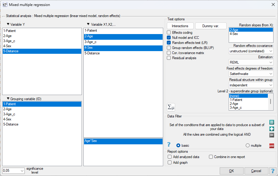
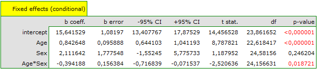
The model converges without a singular fit, even though some children have only 2 measurements – a mixed model does not require complete data. Fixed effects: the intercept 15.64 is the distance of a boy at age 0 (a clinically meaningless extrapolation); age \(b=0.843\) mm/year (\(p<0.000001\)) is the growth rate of boys; sex \(b=2.11\) (\(p=0.246\)) is the difference of girls relative to boys at age 0, again meaningless; the interaction \(b=-0.394\) mm/year (\(t=-2.52\), \(df=24.2\), \(p=0.019\)): girls grow 0.39 mm/year more slowly than boys, i.e. at a rate of \(0.843-0.394=0.449\) mm/year. This is the answer to the research question.
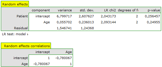
Random effects: the standard deviation of the intercept is 2.61 mm and of the slope 0.24 mm/year, but the correlation between them is \(-0.78\). This does not mean that „larger” children grow more slowly – the intercept refers to age 0, far outside the data range (8–14 years), and with the zero placed there the correlation is an artefact of the geometry of the lines. The LR tests for both components are not significant (\(p=0.256\) and \(p=0.250\)): with 27 children and 2–4 measurements per child, individual growth rates cannot be reliably distinguished, and a model with only a random intercept would be just as good.
Centring age. Let us repeat the analysis, replacing Age with the column Age_c (age \(-11\)) among the \(X\) variables, in the interaction and in the random-slopes list. The model fit (\(-2LL\), AIC) and the coefficients of age and of the interaction remain identical, but the meaning of the intercept and of sex changes: the intercept 24.91 mm is the distance of an average boy at age 11, sex \(b=-2.22\) (\(p=0.006\)) is the difference of girls at age 11 (they are 2.2 mm smaller), and the random-effects correlation changes from \(-0.78\) to \(+0.33\). General conclusion: when the intercept is to be interpretable and the random-effects correlation meaningful, the time (age) variable should be centred in the middle of the observed range.
Example 3. (centresPatients.pqs file)
Simulated data: in 8 centres, 6 patients each had 5 measurements over time (\(t=0,1,\ldots,4\)) of some index \(Y\), with a continuous variable \(X\) also recorded. Patients are nested within centres, so two sources of dependence overlap: measurements of the same patient are alike, and patients of the same centre are alike too.
We indicate \(Y\), the grouping variable Patient, the independent variables t and X, and in the field Level 2 – superordinate group we choose Centre. The grouping variable must be unique across the whole sheet (patient 1 in centre 1 and patient 1 in centre 2 are different people, so they must have different identifiers).
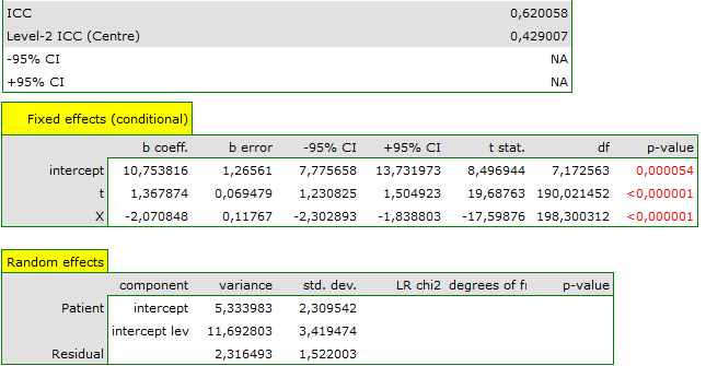
The report shows three variances: patients (5.33), centres (11.69) and residuals (2.32). The null model gives a total ICC of \(0.620\) (62% of the variability consists of differences between patients and centres together) and a level-2 ICC of \(0.429\) (43% of the variability consists of differences between centres alone). Fixed effects: time \(b=1.37\) (\(p<0.000001\)), \(X\): \(b=-2.07\) (\(p<0.000001\)). The degrees of freedom for the intercept are only 7.2 – it is effectively 8 centres that inform us about the overall level, which is why its confidence interval is wide (7.78–13.73) despite 240 observations. A separate level-2 BLUP table identifies centres with an atypical level of \(Y\) (e.g. centre 1: \(-3.86\)).
Example 4. continuation of example 1 (sleepDeprivation.pqs file)
The reaction-time measurements were taken day after day, so the residuals of neighbouring days may be correlated (a bad day drags the next one along). We check this with a model with a random intercept only (no random slope) and the AR(1) residual structure; the rows of each subject are ordered by day in the sheet, which is a requirement of this option.
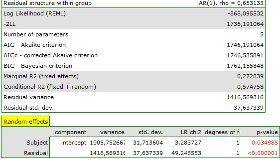
The parameter \(\rho=0.653\): the residuals of two neighbouring days are correlated at 0.65, of days two apart – \(0.65^2\approx0.43\), and so on. The AR(1) model with a random intercept has \(-2LL=1736.19\) and AIC \(=1746.19\), whereas the same model without a residual structure has \(-2LL=1786.47\) and AIC \(=1794.47\) – an enormous improvement. Interestingly, the AIC of the AR(1) model is also lower than that of the random-slope model of example 1 (1755.63; the comparison is allowed because both models have the same fixed effects and are fitted by REML). Both models describe the same phenomenon in a different language: the random slope says „each person has their own constant rate”, AR(1) says „deviations from the line persist for several days”. The effect of day remains almost the same (\(b=10.47\), error 1.34).
Estimation: The parameters are estimated by maximum likelihood (ML) or restricted maximum likelihood (REML; Laird and Ware 1982[188], Bates et al. 2015[184]). The covariance of a group's random effects is parameterized as \(\sigma^2\Lambda\Lambda^T\), where \(\Lambda\) is a lower-triangular matrix (diagonal for the independent covariance). For a fixed \(\Lambda\) the fixed effects and \(\sigma^2\) have a closed form (generalized least squares), and the profiled deviance
(for REML; for ML without the last term and with \(n\) instead of \(n-p\)) is minimized numerically by the Nelder-Mead method. \(A_j=I+\Lambda^TZ_j^TZ_j\Lambda\), \(W\) is the inverse of the marginal covariance matrix, and \(r^2\) is the weighted residual sum of squares. The computations are carried out blockwise, group by group. With an AR(1) or CS residual structure, the products \(Z_j^TZ_j\) and the sums of squares are computed with weights \(R_j^{-1}\), where \(R_j\) is the residual correlation matrix of the group (\(\rho^{|i-i'|}\) for AR(1), a constant \(\rho\) off the diagonal for CS), and \(\rho\) is an additional optimization parameter. A second level of nesting adds a random intercept of the superordinate group with variance \(\tau_{(2)}^2\).
Satterthwaite degrees of freedom: for the \(j\)-th fixed effect \(df_j=2\,\mathrm{Var}(\hat\beta_j)^2/\mathrm{Var}[\mathrm{Var}(\hat\beta_j)]\), where the variance of the variance is computed by the delta method from the Hessian of the deviance with respect to the variance parameters (Kuznetsova et al. 2017[187]).
ICC and its confidence interval: \(ICC=\tau^2/(\tau^2+\sigma^2)\) from the null model; the confidence interval by the delta method from the Hessian of the deviance with respect to \((\tau^2,\sigma^2)\).
Nakagawa's \(R^2\): \(R^2_{marg}=\sigma_f^2/(\sigma_f^2+\sigma_u^2+\sigma^2)\) and \(R^2_{cond}=(\sigma_f^2+\sigma_u^2)/(\sigma_f^2+\sigma_u^2+\sigma^2)\), where \(\sigma_f^2\) is the variance of the fixed-effects prediction and \(\sigma_u^2\) the mean random-effects variance (for random slopes averaged over the values of \(X\)).
LR test on the boundary: the statistic \(2(\ell_1-\ell_0)\) for the hypothesis of zero variance asymptotically follows a 50:50 mixture of \(\chi^2_{q-1}\) and \(\chi^2_q\) (Self and Liang 1987[193]); for one parameter the \(p\)-value from \(\chi^2_1\) is halved.
Group random effects: \(\hat u_j=\Lambda A_j^{-1}\Lambda^TZ_j^T(y_j-X_j\hat\beta)\) with conditional covariance \(\sigma^2\Lambda A_j^{-1}\Lambda^T\) (best linear unbiased predictors, BLUP).