 PQStat
 Mixed logistic regression (generalized linear mixed model)
When to use:
Mixed logistic regression (generalized linear mixed model, GLMM) extends logistic regression to data in which observations form groups: repeated assessments of the same patient (e.g. presence of a symptom at successive visits), patients from the same centre, animals from the same herd, pupils from one class (see the introduction to mixed models). The binary (0/1) outcomes of observations from one group are correlated, and ordinary logistic regression, which ignores this correlation, underestimates standard errors and overstates significance.
The model describes the logit of the probability of the event:
where:
\(Y_{ij}\) – the outcome of the \(i\)-th observation in group \(j\) (0 or 1),
\(\beta_0,\beta_1,\ldots,\beta_k\) – fixed effects,
\(u_{0j}\) – the random intercept of group \(j\), \(u_{1j}\) – the random slope of group \(j\); the random effects are assumed normal with mean 0 and covariance matrix \(\Sigma\) on the logit scale.
A random intercept means that each group has its own „baseline” odds of the event: a group with \(u_{0j}=1\) has odds \(e^{1}\approx2.7\) times higher than an average group, at the same values of the variables. Unlike mixed multiple regression, the model has no residual variance: on the logit scale it is replaced by the constant \(\pi^2/3\approx3.29\).
This model replaces Cochran's Q ANOVA when the repeated measurements are incomplete or when, besides the repeated factor, the model is to contain continuous variables and variables describing the group.
Assumptions
- a binary dependent variable,
- random effects normally distributed on the logit scale; groups independent of one another,
- at least 3 groups, and usually a dozen or more for a reliable variance estimate; with random slopes also several observations in each group,
- a sufficient number of events (ones) and non-events (zeros) – as in logistic regression,
- missing data are random.
Definitions of measures
Conditional odds ratio \(OR=e^{b}\) – says how many times the odds of the event change when \(X\) increases by one unit within the same group (for the same patient, in the same centre). Ordinary logistic regression gives a population odds ratio, averaged over all groups. The conditional OR is always larger in absolute value (further from 1) than the population one, and the difference grows with the random-effect variance; with variance \(\tau^2\) the population coefficient is approximately \(b/\sqrt{1+0.346\,\tau^2}\). Both are correct, but they answer different questions and should not be compared directly.
Random-effect variance \(\tau^2\) on the logit scale and its square root – the standard deviation. A random-intercept standard deviation of 1 means that a group one deviation above average has odds of the event \(e^{1}\approx2.7\) times higher than an average group, and the extreme groups (\(\pm2\) deviations) differ in odds by \(e^{4}\approx55\) times.
ICC on the logit scale – from the null model:
interpreted as the correlation of the latent propensities to the event within a group (the share of between-group variability in the variability of the latent continuous variable behind the 0/1 outcome).
Marginal and conditional \(R^2\) (Nakagawa) – on the logit scale, with \(\pi^2/3\) as the residual variance: the share of variance explained by the fixed effects, and by the fixed and random effects together.
Likelihood approximation – the likelihood of the model requires integration over the random effects, which cannot be done exactly. Laplace approximates the integral by a single function around its maximum – fast and sufficiently accurate with larger groups. Gauss-Hermite quadrature (adaptive, 7, 15 or 25 nodes) computes the integral numerically at several points and is more accurate, especially with small groups (a few observations per group) and a large variance; the cost is computation time. Quadrature is available only for a model with a random intercept alone; with random slopes the program uses the Laplace approximation. The results of the different approximations usually differ in the third significant digit.
LR test of random effects, BLUP, singular fit – as in mixed multiple regression; the BLUPs are group deviations on the logit scale.
Conditional and population prediction – the predicted probability with the group's random effects („for this patient”) and from the fixed effects alone („for the average patient”). Classification and the ROC curve can be computed for both; the conditional prediction is always more accurate, because it uses information about the group, but it cannot be used for new, unknown groups.
How to set up the analysis
Statistics \(\to\) Mixed models \(\to\) Mixed logistic regression.
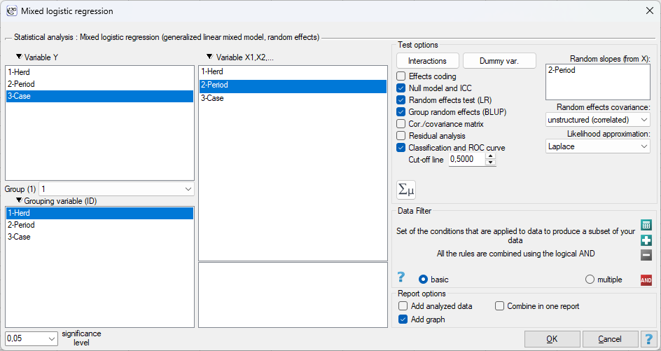
In the window we indicate the Dependent variable Y and, in the Group (1) field, the value denoting the event, the Grouping variable (ID) and the Independent variables X1, X2, …; dummy variables and interactions are prepared as in logistic regression. Mixed-model options:
- Random slopes (from X) – variables among \(X\) whose effect is to differ between groups; they must vary within groups. The random intercept is always in the model. Random slopes in a logistic model require more observations per group than in a linear model, because each observation carries only one bit of information,
- Random effects covariance – unstructured (correlated) or independent; the latter is more stable with few groups,
- Likelihood approximation – Laplace (default, always available) or G-H quadrature with 7, 15 or 25 nodes (random intercept only). Changing the approximation slightly changes all numbers in the report; for publication, with small groups, quadrature with 15–25 nodes is worth using,
- Null model and ICC, Random effects test (LR), Group random effects (BLUP), Cor./covariance matrix, Residual analysis – as in mixed multiple regression,
- Classification and ROC curve – sensitivity, specificity, fraction correct and AUC for the indicated cut-off, separately for the conditional and population prediction,
- Add graphs – the caterpillar plot of group random effects.
Results and interpretation
Counts – number of observations, count of \(Y=1\), number of groups, minimum, median and maximum of observations per group. With a median below 3 observations per group the Laplace approximation is least accurate – quadrature is then worth using.
Approximation and convergence – method (Laplace or Gauss-Hermite with the number of nodes), number of iterations, convergence, singular fit.
Model fit – log-likelihood, \(-2LL\), AIC, AICc, BIC (ML estimation), marginal and conditional \(R^2\) and – for comparison – the \(-2LL\) of ordinary logistic regression (no random effects) and the \(-2LL\) of the null model.
LR test of random effects (vs logistic regression) – whether the group structure is needed; the \(p\)-value is boundary-corrected.
Null model – between-group variance \(\tau^2\) and the ICC (logit scale) with its confidence interval.
Fixed effects (conditional) – \(b\), error, confidence interval, the \(z\) statistic, the \(p\)-value and the odds ratio (conditional) with its confidence interval. The test is a Wald \(z\)-test (no degrees of freedom), as in logistic regression.
Random effects – the variance and standard deviation of each component on the logit scale, LR tests of the need for the components; the last row is the constant \(\pi^2/3\). With more than one component – the random-effects correlation matrix.
Group random effects (BLUP) – deviations of the groups from the population on the logit scale with errors. A group with BLUP \(=0.5\) has odds of the event \(e^{0.5}\approx1.65\) times higher than an average group. Groups with few observations or without events have their BLUPs shrunk towards zero.
Classification and ROC curve – for the conditional prediction (with BLUP) and the population prediction: sensitivity, specificity, fraction correct, AUC with its error and confidence interval. The AUC difference between them shows how much discriminating ability knowledge of the group adds.
Residual analysis – the conditional and population predicted probability and Pearson residuals for each observation.
Execution and interpretation
Example 1. (herdsCBPP.pqs file)
In a study of contagious bovine pleuropneumonia (CBPP) in Ethiopia (Lesnoff et al. 2004[189]), 15 zebu herds were observed over four consecutive periods. For each animal in each period it was recorded whether a new case of the disease appeared. The data are in long format: Herd (1–15), Period (1–4) and Case (1 – new case, 0 – none); 842 observations, including 99 cases, from 26 to 96 observations per herd. We ask whether the incidence changes over successive periods of the epidemic and how much the herds differ from one another.
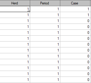
Animals from one herd share conditions, contacts and immunity, so their outcomes are not independent – the herd is the natural grouping variable. We build the model: Case as \(Y\) with the value 1 in the Group (1) field, Herd as the grouping variable, Period as the independent variable. Period is a qualitative variable with four categories, so with the Dummy variables button we convert it into three dummy variables with period 1 as the reference category. We keep the random intercept only (period has no random slope), the Laplace approximation, and switch on Null model and ICC, Random effects test (LR), Group random effects (BLUP), Classification and ROC curve and Add graphs.
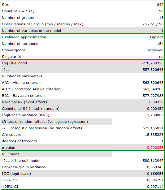
Step 1 – fit. 842 observations, 99 events, 15 groups (26/61/96 observations per group), convergence achieved, no singular fit. The \(-2LL\) of the model is 555.00 (AIC \(=565.00\)), whereas ordinary logistic regression with the same variables has \(-2LL=569.01\). LR test of random effects: \(\chi^2=14.01\), \(df=1\), \(p=0.00009\) (boundary-corrected) – the herds differ significantly in incidence, and a model without the random effect would be invalid.
Step 2 – ICC. In the null model the between-herd variance is 0.659, hence ICC \(=0.659/(0.659+3.29)=0.167\) (95% CI: 0.037–0.297): about 17% of the latent variability of the propensity to fall ill consists of differences between herds.

Step 3 – fixed effects. The intercept \(b_0=-1.399\) corresponds to a probability of falling ill in period 1 in an average herd of \(1/(1+e^{1.399})=0.198\). Conditional odds ratios for the successive periods relative to period 1: period 2 – \(OR=0.371\) (95% CI: 0.203–0.676, \(p=0.0012\)), period 3 – \(OR=0.324\) (0.171–0.614, \(p=0.0005\)), period 4 – \(OR=0.206\) (0.089–0.476, \(p=0.0002\)). Within the same herd the odds of a new case in period 2 are 63% lower than in period 1, and in period 4 – 79% lower: the epidemic is dying out. The word „conditional” reminds us that we compare periods within a herd; the odds ratio averaged over all herds (from ordinary logistic regression) would be somewhat closer to 1.

Step 4 – random effects. The random-intercept variance is 0.413, the standard deviation 0.642 on the logit scale. A herd one deviation above average has odds of disease \(e^{0.642}\approx1.9\) times higher than an average herd, and the difference between the extreme herds (\(\pm2\) deviations) is a \(e^{2.57}\approx13\)-fold difference in odds. Marginal \(R^2=0.088\), conditional \(=0.190\): period explains less than 9% of the variability on the logit scale, and together with herd – 19%.
[obraz: ANG_raport_mixed_log_blup.png]
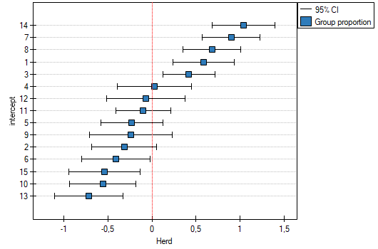
Step 5 – atypical herds. The BLUP of herd 1 is \(+0.590\) (error 0.348): its odds of disease are \(e^{0.59}\approx1.8\) times higher than those of an average herd; in period 1 this gives a probability of \(1/(1+e^{1.399-0.590})=0.308\) instead of 0.198. Herd 2 has BLUP \(-0.299\) (odds 26% lower). The caterpillar plot orders the herds from the least to the most at risk; herds whose interval does not include zero clearly depart from the average. Bear in mind that herds with few animals have their BLUPs shrunk towards zero.

Step 6 – classification. The classification and ROC table shows two versions: the conditional prediction (with the herd's BLUP) and the population prediction (period only). The AUC of the conditional prediction is higher – knowing the herd improves the discrimination between animals that will and will not fall ill. The population version says how the model will perform in a new, unknown herd.
What the approximation changes. The same model with G-H quadrature, 25 nodes gives \(-2LL=554.92\), a herd variance of 0.419 instead of 0.413 and coefficients differing in the third decimal place (e.g. period 4: \(b=-1.579\) instead of \(-1.580\)). With herds of 26–96 animals the Laplace approximation is fully sufficient; if the groups had 2–3 observations each, the differences would be larger and quadrature would become the method of choice.
Estimation: The marginal likelihood requires integration over the random effects, which has no closed form. The program uses the Laplace approximation (Bates et al. 2015[184]): for each group it finds the mode \(\hat u_j\) of the penalized log-likelihood
and approximates the deviance by \(\sum_j\left[2f_j(\hat u_j)+\ln\det(I+\Lambda^TZ_j^TW_jZ_j\Lambda)\right]\), where \(W_j\) is the matrix of weights \(p(1-p)\) and \(\Sigma=\Lambda\Lambda^T\). For a single random component the integral can be computed by adaptive Gauss-Hermite quadrature around the mode, with nodes shifted and scaled according to the mode and curvature of each group. The parameters \((\theta,\beta)\) are optimized jointly by the Nelder-Mead method, starting from logistic regression.
Standard errors: from the inverse of the Hessian of the deviance with respect to all parameters \((\theta,\beta)\), computed numerically at the optimum, as in the lme4 package.
ICC: \(\tau^2/(\tau^2+\pi^2/3)\) from the null model, with a delta-method confidence interval.
Nakagawa's \(R^2\): as in mixed multiple regression, with \(\pi^2/3\) in place of the residual variance.
Test on the boundary: the statistic \(2(\ell_1-\ell_0)\) for the hypothesis of zero variance follows a 50:50 mixture of \(\chi^2_{q-1}\) and \(\chi^2_q\) (Self and Liang 1987[193]); for one parameter the \(p\)-value from \(\chi^2_1\) is halved.
Population effect: with a random intercept of variance \(\tau^2\) the population (marginal) coefficient is approximately \(\beta/\sqrt{1+0.346\,\tau^2}\) (Zeger et al. 1988[195]).