 PQStat
 Validation and prediction for mixed multiple regression
When to use:
A built and verified mixed model can be used for prediction of \(Y\) for new data and for validation on a test set, as in validation and prediction for multiple regression. A mixed model, however, allows two kinds of prediction:
- population prediction – from the fixed effects alone (random effects equal to 0); it answers the question „what value do we expect for an average, new group (patient, centre)”;
- group prediction – from the fixed effects and the random effect (BLUP) of a specific group that took part in building the model; it answers the question „what value do we expect for this patient (in this centre)”. It is more accurate, but available only for groups known to the model.
For new observations whose identifier did not occur in the training data, the program always uses population prediction.
How to set up the analysis
Statistics \(\to\) Mixed models \(\to\) Mixed multiple regression – prediction/validation.
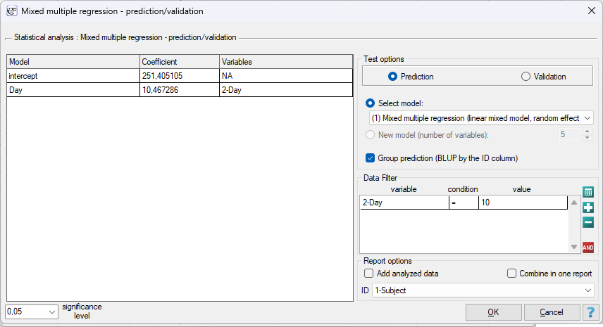
Prediction requires a model saved in the program (a mixed multiple regression report assigned to the sheet), because besides the coefficients the group random effects and the covariance matrix are needed; coefficients cannot be entered by hand. After the model is chosen, the program fills in the list of variables, and we indicate the sheet columns with the new values of \(X\). Options:
- Group prediction (BLUP by the ID column) – after ticking it we indicate the column with the group identifier; for identifiers known to the model the prediction includes the group's BLUP, for the others it is population prediction. Without this option all predictions are population predictions;
- validation – when the new data contain an observed \(Y\), we indicate it, and the report contains measures of the model's fit to the test set.
The data for prediction are placed in the same sheet as the training data (e.g. in subsequent rows), and the analysis is restricted with a filter.
Results and interpretation
The report states which kind of prediction was used (population or for groups), the number of observations for which the group BLUP was used, and for each observation the predicted \(Y\) with its confidence interval. The interval of the population prediction is wider than that for a known group, because it includes the uncertainty about the level of the new group. In validation mode the prediction errors and fit measures are additionally computed.
Example 1. continuation of example 1 (sleepDeprivation.pqs file)
Based on the model with a random intercept and a random slope of day, we want to predict the reaction time on the tenth day of deprivation (day \(=10\), i.e. one day beyond the study range) for subject 308, for subject 309 and for a new, unknown person. We add three rows to the sheet with the value 10 in the Day column and the identifiers 308, 309 and 999, then run the prediction with a filter on these rows and the Group prediction option on.
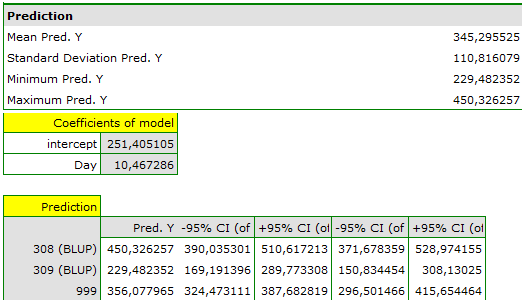
For the new person (999) the prediction is the population one: \(251.41+10.47\cdot10\approx356\) ms. For subject 308 the program adds their random effects (intercept \(+2.26\), slope \(+9.20\)): \((251.41+2.26)+(10.47+9.20)\cdot10\approx450\) ms, and for subject 309 (effects \(-40.40\) and \(-8.62\)): \((251.41-40.40)+(10.47-8.62)\cdot10\approx230\) ms. The difference between subjects 308 and 309 reaches 220 ms, although at the population level both „should” have 356 ms – this illustrates how much information the random effects carry when the group is known. The confidence interval of the population prediction is at the same time the widest, because it includes the scatter between people.