 PQStat
 Validation and prediction for mixed logistic regression
When to use:
A built model can be used for prediction of the probability of the event for new observations and for validation on a test set, as in validation and prediction for logistic regression. As in mixed multiple regression, two kinds of prediction are available:
- population – from the fixed effects alone; the probability for an average, unknown group,
- for a group – with the random effect (BLUP) of a group known to the model; the probability for this specific patient, centre, herd.
Prediction of the occurrence of the event (1) or its absence (0) consists in comparing the predicted probability with the cut-off point (0.5 by default).
How to set up the analysis
Statistics \(\to\) Mixed models \(\to\) Mixed logistic regression – prediction/validation.
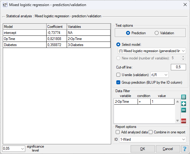
We indicate a model saved in the program (a mixed logistic regression report assigned to the sheet) – entering coefficients by hand is not possible, because the group random effects are needed. Then we indicate the columns with the new values of the variables, optionally the observed \(Y\) (validation) and the option Group prediction (BLUP by the ID column) with the identifier column. For identifiers unknown to the model the prediction is the population one.
Results and interpretation
The report states the kind of prediction, the number of observations for which the group BLUP was used, and for each observation the predicted probability and the predicted class. In validation mode additionally the classification (sensitivity, specificity, fraction correct) and the AUC on the test set.
Example 1. continuation of example 1 (wardsInfections.pqs file)
Based on the surgical site infection model (operation time and diabetes as fixed effects, a random ward intercept and a random slope of operation time), we want to estimate the risk of infection for a diabetic patient whose operation lasted one standard deviation longer than average (OpTime \(=1\), Diabetes \(=1\)), if operated in ward 1, in ward 2, or in a new ward unknown to the model.
First we build and save the model in the Mixed logistic regression window: Infection as \(Y\) (Group (1) \(=1\)), Ward as the grouping variable, OpTime and Diabetes as \(X\), OpTime in the random-slopes list, unstructured covariance, with the Group random effects (BLUP) option on. Then we add three rows to the sheet with the values 1 and 1 in the OpTime and Diabetes columns and ward identifiers 1, 2 and 99, set a filter on these rows, and in the prediction window indicate the saved model and the Group prediction (BLUP by the ID column) option with the Ward column.
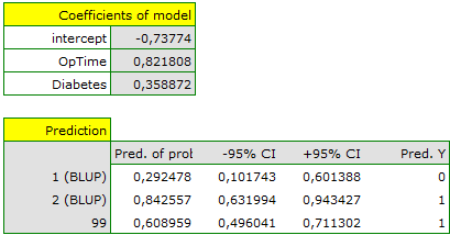
Fixed effects of the model: intercept \(-0.738\), operation time \(0.822\), diabetes \(0.359\); BLUP of ward 1: intercept \(-1.145\), slope \(-0.182\); of ward 2: \(+1.193\) and \(+0.041\). For the new ward (99) the prediction is the population one: logit \(=-0.738+0.822+0.359=0.443\), probability \(0.61\). For ward 1 the program adds its intercept and slope BLUPs (the latter multiplied by the operation time): logit \(=0.443-1.145-0.182\cdot1=-0.884\), probability \(0.29\). For ward 2: logit \(=0.443+1.193+0.041=1.677\), probability \(0.84\). The same patient thus has a risk of infection from 29% to 84% depending on the ward, and the population prediction (61%) is merely the middle of this range. With a cut-off of 0.5 the patient in ward 1 would be classified as „no infection”, in ward 2 and in the new ward – as „infection”. In validation mode (with the Infection column indicated) on a test set the report would additionally give sensitivity, specificity and AUC.