 PQStat
 Cox PH regression with random effect (frailty)
When to use:
The Cox model with random effect extends Cox proportional hazards regression to data in which observations form groups: patients treated in the same centre, animals from one litter, recurrent events in the same patient (successive infections, successive hospitalizations), the eyes or kidneys of the same patient (see the introduction to mixed models). Survival times within a group are related, because the group shares unobserved risk factors: a patient has their own immunity, a centre – its own quality of care. Ordinary Cox regression ignores this dependence, which underestimates the standard errors of the coefficients and overstates significance.
The random effect, called frailty in survival analysis, is an unobserved factor \(w_j\) shared by the whole group \(j\), which multiplies the hazard of each of its observations:
where:
\(h_{ij}(t)\) – the hazard of the \(i\)-th observation in group \(j\),
\(h_0(t)\) – the baseline hazard,
\(\beta_1,\ldots,\beta_k\) – coefficients (fixed effects),
\(w_j\) – the frailty of group \(j\); a gamma distribution with mean 1 and variance \(\theta\) is assumed (shared gamma frailty).
Groups with \(w_j>1\) have a higher risk than their variables imply, groups with \(w_j<1\) – a lower one. The variance \(\theta\) says how much the groups differ in risk; \(\theta=0\) means no within-group dependence, and the model reduces to ordinary Cox regression. Frailty is the counterpart of the random intercept of mixed multiple regression, except that it acts multiplicatively on the hazard; random slopes are not available in this model.
Assumptions
- proportional hazards, as in Cox regression,
- groups independent of one another; dependence occurs only within groups,
- at least 3 groups, and usually a dozen or more for a reliable estimate of \(\theta\),
- a sufficient number of events (complete observations); groups without events carry little information about \(\theta\),
- no strong collinearity of the independent variables.
Definitions of measures
Frailty variance \(\theta\) – a measure of the differentiation of risk between groups. Frailty has mean 1, so with \(\theta=0.4\) the standard deviation of \(w_j\) is \(\sqrt{0.4}\approx0.63\): a typical group has a hazard 60% higher or lower than its variables would imply. The error of \(\theta\) is approximate (from the profile likelihood) and is not meant for testing – the LR test serves that purpose.
Kendall's \(\tau\) – a measure of the dependence of the survival times of two observations from the same group, following from the gamma distribution:
\(\tau=0\) is independence; \(\tau=0.17\) means moderate concordance: an observation from a group in which another observation survived long has itself a better chance of surviving long.
LR test: \(\theta=0\) – a likelihood ratio test comparing the frailty model with ordinary Cox regression. The hypothesis lies on the boundary of the parameter space, so the \(p\)-value from \(\chi^2_1\) is halved (boundary correction), which the report states.
Conditional hazard ratio \(HR=e^{b}\) – how many times the hazard changes when \(X\) increases by one unit within the same group (at the same frailty). The population HR from ordinary Cox regression is averaged over groups and is closer to 1 in absolute value; the two should not be compared directly.
Group random effects – the estimated \(w_j\) for each group and \(\log w_j\) with its error. Groups with few events have their \(w_j\) shrunk towards 1 (we do not know enough about them to call them atypical). Their significance is not tested; they serve to identify groups with elevated or reduced risk.
Integrated likelihood – the log-likelihood of the model after integrating out the frailty; the information criteria and LR tests (both the test of \(\theta=0\) and the test of the joint effect of the independent variables) are based on it.
How to set up the analysis
Statistics \(\to\) Mixed models \(\to\) Cox PH regression with random effect.
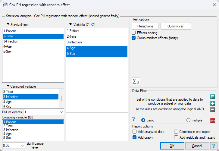
The window has the layout of the Cox regression window. We indicate the Survival time, the Censoring variable with the value denoting the event in the Complete field, and the Independent variables X1, X2, …; dummy variables and interactions are prepared exactly as in Cox regression. Options of the random-effect model:
- Grouping variable (ID) – the column indicating the group of the observation (centre, patient, litter); numeric or text. It is mandatory – without it the model does not differ from Cox regression,
- Group random effects (frailty) – adds to the report a table of the estimated \(w_j\) for each group; with hundreds of groups the table is long,
- Add residuals and hazard – martingale and deviance residuals accounting for the frailty, and the resulting hazard \(w_j H_i\) of each observation; they serve to assess the fit and identify outlying observations,
- Add graphs – group survival curves (frailty).
Tied times are handled by the Breslow method, as in Cox regression, so with \(\theta=0\) the results of both analyses are identical.
Results and interpretation
Counts – the number of observations, complete (events) and censored, and the number of groups. The report also recalls the sample-size condition \(n\ge10k/p\) known from Cox regression.
Model fit – the integrated log-likelihood of the model, the same quantity for the model with the random effect only (no variables), and the likelihood ratio test of the joint effect of the independent variables. The information criteria AIC, AICc, BIC and pseudo-\(R^2\) as in Cox regression.
Random effect (gamma frailty) – grouping variable, number of groups, frailty variance \(\theta\) with an approximate error (profile), Kendall's \(\tau\) and the LR test: \(\theta=0\) (vs Cox regression) with boundary correction. A significant result means that the group structure must not be ignored. The number of EM iterations is also given.
Coefficients – \(b\), error, confidence interval, Wald statistic, \(p\)-value and the hazard ratio (conditional) \(HR=e^{b}\) with its confidence interval. The standard errors come from the penalized information matrix and account for the presence of the random effect, which is why they are larger than in ordinary Cox regression.
Baseline functions – cumulative hazard and survival for an average group (\(w_j=1\)): at the mean values of the variables and baseline, as in Cox regression.
Group random effects (gamma frailty) – for each group: \(w\), \(\log w\) with its error, number of events, size and the cumulative hazard of the group. A group with \(w=1.4\) has a hazard 40% higher than an average group with the same variables; a group with \(w=0.6\) – 40% lower. Groups with many events at a small expected cumulative hazard receive \(w>1\), groups without events despite long observation – \(w<1\).
Graphs – Group survival curves (frailty): the survival curve for an average group (\(w=1\)) and for selected groups with their frailty; the higher \(w\), the lower the curve lies.
Execution and interpretation
Example 1. (kidneyCatheter.pqs file)
In the study of McGilchrist and Aisbett (1991)[190], 38 dialysis patients with an inserted catheter were observed. The time (in days) to infection at the catheter insertion site was recorded; after the infection was cured the catheter was reinserted, so each patient has two episodes. The catheter was sometimes removed for other reasons – such observations are censored. Data in long format: Patient (1–38), Time (days), Infection (1 – infection, 0 – censored observation), Age (years) and Sex (0 – male, 1 – female). In total 76 observations, 58 infections. We ask whether age and sex affect the risk of infection and whether patients differ in their individual susceptibility.
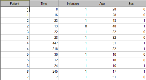
Two episodes of the same patient are not independent – the patient has their own immunity, hygiene, comorbidities. If we fitted ordinary Cox regression, we would treat 76 episodes as 76 different people. We therefore build a model with a random effect: Time as the survival time, Infection as the censoring variable with the value 1 as Complete, Age and Sex as independent variables, Patient as the grouping variable. We switch on Group random effects (frailty) and Add graphs.
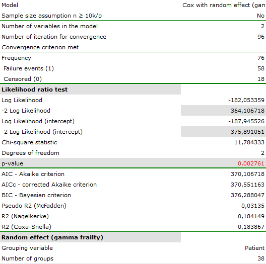
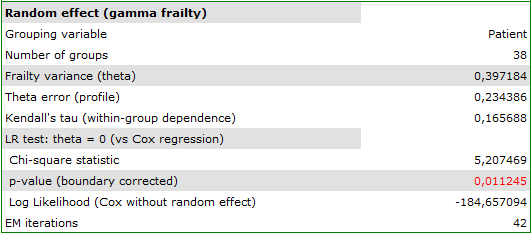
Step 1 – do patients differ in susceptibility. Frailty variance \(\theta=0.397\) (error 0.234), Kendall's \(\tau=0.166\). LR test \(\theta=0\): \(\chi^2=5.21\), \(p=0.011\) (boundary-corrected) – ordinary Cox regression is not valid for these data; patients differ significantly in their unobserved susceptibility to infection. The frailty standard deviation \(\sqrt{0.397}\approx0.63\): a typical patient has a hazard of infection about 60% higher or lower than their age and sex imply.
Step 2 – fit. The integrated log-likelihood of the model is \(-182.05\), of the model with frailty only (no variables) \(-187.95\); LR test of the joint effect of the variables: \(\chi^2=11.78\), \(df=2\), \(p=0.0028\). AIC \(=370.11\).

Step 3 – coefficients. Age: \(b=0.0055\), \(HR=1.006\) (95% CI: 0.983–1.029), \(p=0.637\) – age does not affect the risk of infection. Sex: \(b=-1.556\) (error 0.445), \(HR=0.211\) (95% CI: 0.088–0.504), \(p=0.0005\). The hazard of infection in women is 79% lower than in men – when compared within the same „susceptibility”, i.e. conditionally. The error of the sex coefficient (0.445) is larger than ordinary Cox regression would give, because the model takes into account that the information from two episodes of the same patient partly repeats itself.
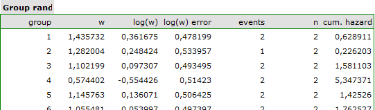
Step 4 – atypical patients. The group random effects table: patient 1 has \(w=1.44\) (\(\log w=0.36\), error 0.48) – two infections at a small expected cumulative hazard (0.63) mean a susceptibility 44% above average. Patient 4 has \(w=0.57\): also two infections, but at a large cumulative hazard (5.35), i.e. after a long observation – their susceptibility is 43% below average. The errors of \(\log w\) (about 0.5) are large, because each patient has only two episodes; the frailties of individual patients should be treated as indicative.
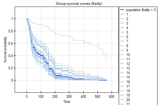
The group survival curves graph shows the curve for an average patient (\(w=1\)) and the curves of patients with higher and lower frailty: patient 1 loses „infection-free survival” faster, patient 4 – more slowly.
Estimation: The parameters are estimated by the EM algorithm on the profiled partial likelihood (Klein 1992[186], Therneau and Grambsch 2000[194]). In the M step a Cox regression with the offset \(\log w_j\) is fitted and the Breslow cumulative baseline hazard \(H_0(t)\) is determined; in the E step the frailty of a group is replaced by its expected value
where \(D_j\) is the number of events in the group and \(A_j\) its cumulative hazard. The variance \(\theta\) is determined by maximizing the integrated log-likelihood
which as \(\theta\to0\) turns into the Cox partial likelihood (\(D\) – the total number of events). Convergence is accepted when the change of \(\ell\) is smaller than \(10^{-9}\).
Standard errors: from the penalized information matrix for the parameters \((\beta,\log w_1,\ldots,\log w_G)\), where the penalty follows from the gamma distribution; the \(\beta\) block is inverted through the Schur complement.
Kendall's \(\tau\): for shared gamma frailty \(\tau=\theta/(\theta+2)\).
Test on the boundary: the statistic \(2(\ell_{frailty}-\ell_{Cox})\) asymptotically follows a 50:50 mixture of a distribution degenerate at zero and \(\chi^2_1\) (Self and Liang 1987[193]), which is why the \(p\)-value from \(\chi^2_1\) is halved.